BSM2 in Collimator
A markdown file converted from Vannary's notes in
DOCXformat
Priority Lists
Get Brian's input on how I should approach building the controller (set up a document with a screenshot and send to Brian on Slack)
Finish the rest of submodels (5 main submodels)
Multi-variance time series
Parameter indexes between MATLAB and Collimator
| Variables | MATLAB index | MATLAB C index | Collimator | collimator index |
|---|---|---|---|---|
| time | ||||
| Si | 1 | 0 | Soluble | 0 |
| Ss | 2 | 1 | Soluble | 1 |
| Xi | 3 | 2 | Particulate | 0 |
| Xs | 4 | 3 | Particulate | 1 |
| Xbh | 5 | 4 | Particulate | 2 |
| Xba | 6 | 5 | Particulate | 3 |
| Xp | 7 | 6 | Particulate | 4 |
| So | 8 | 7 | Soluble | 2 |
| Sno | 9 | 8 | Soluble | 3 |
| Snh | 10 | 9 | Soluble | 4 |
| Snd | 11 | 10 | Soluble | 5 |
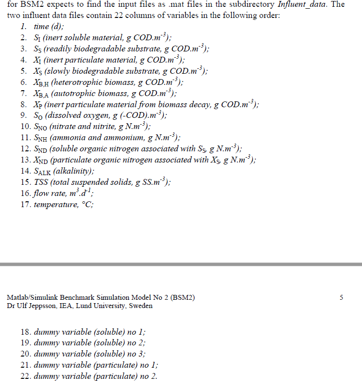
| Xnd | 12 | 11 | Particulate | 5 |
| Salk | 13 | 12 | Soluble | 6 |
| TSS | 14 | 13 | Particulate | 6 |
| Q | 15 | 14 | Q | |
| T | 16 | 15 | T |
Introduction
The benchmark is a simulation environment defining a plant layout, a simulation model, influent loads, test procedures and evaluation criteria. There are multiple vesion of BSM:
- BSM1: combines nitrification with pregentrification, which is most commonly used for nitrogen removal. The control strategies are evaluated over periods of 14 days, with different weather conditions.
- BSMLT: based on BSM1 but with a longer evaluation period (609 days)
BSM2: include BSM1 for the biological treatment of wastewater. The sludge treatment is taken into account.
Extension of BSM2
MATLAB files are available on request by contact Prof Ulf Jeppsson (ulf.jeppsson@iea.lth.se)
Default time unit on Collimator simulations is \'seconds\'
BSM2
2.1. General characteristics
The plant is designed for an average influent dry-weather flow rate of 20,648.36 m3.d-1 and an average
biodegradable COD in the influent of 592.53 g.m-3. Its hydraulic retention time (based on average dry weather
flow rate and total tank volume -- i.e. primary clarifier (900 m3) + biological reactor (12,000 m3) + secondary
clarifier (6,000 m3) -- of 18,900 m3) is 22 hours.
The influent dynamics are defined for 609 days by means of a single file, which takes into account rainfall effect
and temperature.
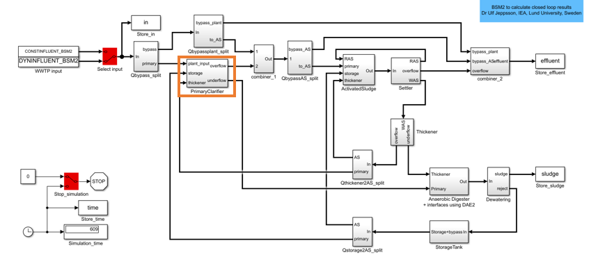 {width="6.5in" height="3.8881944444444443in"}
Note that for the BSM2 system there is rule saying that all influent flow above 60000 m\^3/d should be bypassed.
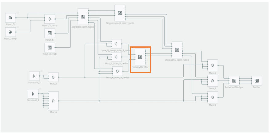 {width="6.5in" height="3.225in"}
Import Input to Collimator
To read your data on Collimator:
Prepare your CSV file:
a. You csv file cannot has more than 4 columns
b. There should not be any space between each value and comma
c. The first row can be used as column header
d.
 {width="2.8676345144356956in"
height="2.969368985126859in"}
{width="2.8676345144356956in"
height="2.969368985126859in"}
Figure 1. Example of CSV file
 {width="5.130627734033246in"
height="1.333086176727909in"}
{width="5.130627734033246in"
height="1.333086176727909in"}
Figure 2. List of CSV files imported to collimator
Upload your CSV file to Collimator inside your project directory
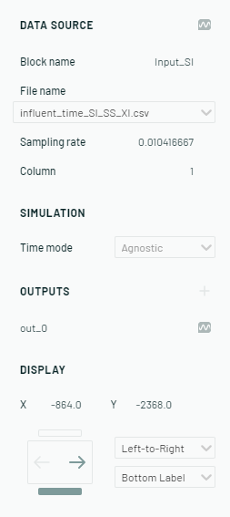
Data Source block is used to import the data from CSV file
a. Select your csv file from file name
b. Entering the sampling rate (what is the time step between your two data points)
c. Column: enter 0 if you want to read data from first column, 1 if you want to read data from the second column and so on.
 {width="1.5470363079615048in"
height="3.4670734908136485in"}
{width="1.5470363079615048in"
height="3.4670734908136485in"}
Figure 3. Data Source block parameter
 {width="0.9238199912510936in"
height="4.019596456692914in"}
{width="0.9238199912510936in"
height="4.019596456692914in"}
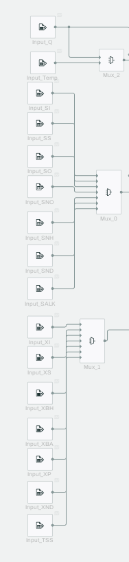
Figure 4. Each influent data needed to import to Collimator individually
 {width="3.881221566054243in"
height="4.188485345581802in"}
{width="3.881221566054243in"
height="4.188485345581802in"}
Constrictions:
Submodels:
There might be discrepancy between the index used to refer to a variable.
File written in C. Index starts with 0
File written in Matlab. Index starts with 1
Hyddelayv3_bsm2
 {width="5.0in" height="1.4895833333333333in"}
Initial condition (XINITDELAYPRIMARY)
- Default value (unit: g/day)
 {width="6.5in" height="0.42083333333333334in"}
Parameters:
T = time constant = 0.0001
PAR1
 {width="2.3031824146981625in"
height="0.46628937007874016in"}
{width="2.3031824146981625in"
height="0.46628937007874016in"}
For state-space system:
U= input; X = state variable; y = output
Input:
Input for soluble block (u) = Si, Ss, So, Sno, Snh, Snd, Salk; Q
Input for particulate block (u) = Xi, Xs, Xbh, Xba, Xp, Xnd, TSS; Q
Input for flow and temperature (u) = Q and Temperature
ODE:
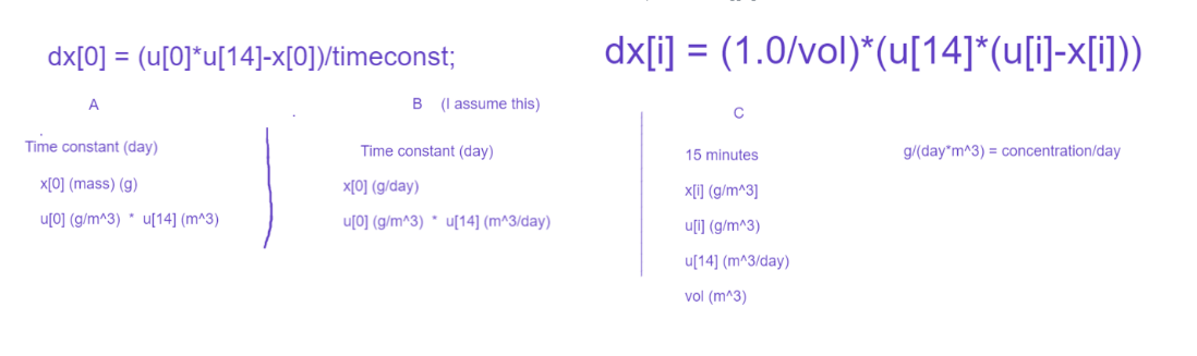
for soluble block: dx = (u*u[Q] -- x)/T
for particulate block (Except for TSS):
other: dx = (u*u[Q]-x)/T
TSS: dx = (u*u[Q] -- x)/T
For flow: dx = (u-x)/T
For temperature: dx = (u-x)/T
Output:
Soluble block: y = x/x[Q]
Particulate block except for TSS: y = x/x[Q]
TSS: y = (X_I2TSS*x[Xi] + X_S2TSS*x[Xs] + X_BH2TSS*x [Xbh] + X_BA2TSS*x [Xba]+X_P2TSS*x [Xp])/x[Q]
Flow: y = x
Temperature: y= x
Primary Clarifier
Initial condition (XINIT_P)
- Default value (unit: g/m\^3)
 {width="6.5in" height="0.4166666666666667in"}
Parameters:
Par_P:
rho = Par_P[0] = Settler efficiency correction = 0.65
K = Par_P[1] = Average COD part/COD tot ratio = 0.85
t_m = Par_P[2] = time to mix = 0.125
f_PS = Par_P[3] = Ratio of primary sludge flow rate to the influent flow = 0.007
VOL_P:
- Vol = Volume of Primary Clarify = 900
XVEKTOR_P (Settleable: 0 = not settle, 1 = settle):
{width="5.595457130358705in" height="0.3634656605424322in"}
- PAR1
{width="2.3031824146981625in"
height="0.46628937007874016in"}
For state-space system:
U= input; X = state variable; y = output
Inputs:
Input for soluble block (u) = Si, Ss, So, Sno, Snh, Snd, Salk; Q
Input for particulate block (u) = Xi, Xs, Xbh, Xba, Xp, Xnd, TSS; Q
Input for flow and temperature (u) = Q and Temperature
ODE:
for soluble block: dx = u[Q]/vol * (u-x)
for particulate block (Except for TSS):
other: dx = u[Q]/vol*(u-x)
TSS: dx = 0
For flow: dx = (u-x)/t_m
For temperature: dx = u[Q]/vol*(u-x)
Outputs:
Parameters (calculate using python script block)
Qu = underflow from PC = f_PS*u[Q]
E = thickening factor = u[Q]/Qu
tt = vol/(x[Q]+0.001) = hydraulic retention time within primary clarifier
nCOD = rho*(2.88*K-0.118)*(1.45+6.15*log(tt*24.0*60.0)) = Total COD removal efficiency in primary clarifier in %
nX = nCOD/K = removal efficiency for particulate COD in % since assumption that soluble COD is not removed. (have be between [0,100])
Soluble block:
Effluent: y = x
Primary Sludge: y = x
Particulate block except for TSS:
Parameter:
- ff = (1.0 -- nX/100.0)
Effluent: y = ff*x
Primary Sludge: y = ((1.0-ff)*E + ff)*x
TSS:
Effluent:
- y = X_I2TSS*y_effluent[Xi] + X_S2TSS*y_effluent [Xs] + X_BH2TSS*y_effluent [Xbh] + X_BA2TSS*y_effluent [Xba]+X_P2TSS*y_effluent [Xp]
Primary Sludge:
- y = X_I2TSS*y_primarysludge[Xi] + X_S2TSS*y_primarysludge [Xs] + X_BH2TSS*y_primarysludge [Xbh] + X_BA2TSS*y_primarysludge [Xba]+X_P2TSS*y_primarysludge [Xp]
Flow:
Effluent: y = u[Q]-Qu
Primary Sludge: y = Qu
Temperature:
Effluent: y = x
Primary Sludge: y = x
Block used in Collimator:
- FlowCombiner3 is used to find the new flow concentration of the combined flow from plant input, storage, and thickener tank.
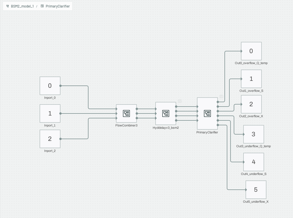 {width="5.0in" height="3.7291666666666665in"}
PC_S -- calculate the concentration of the soluble materials of the flow exiting the PC
PC_X_Q -- calculate the concentration of the particulate materials of the flow and the flow rate exiting the PC
PC_temp -- calculate the temperature of the flow exiting the pC
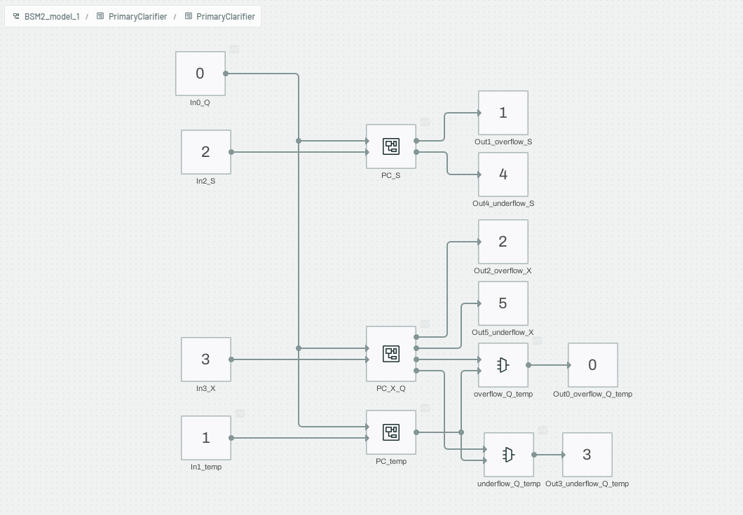 {width="5.0in" height="3.46875in"}
- Inside PC_S submodel. The output concentration is equal to the state of concentration at time i. The integrator block is used to solve ODE.
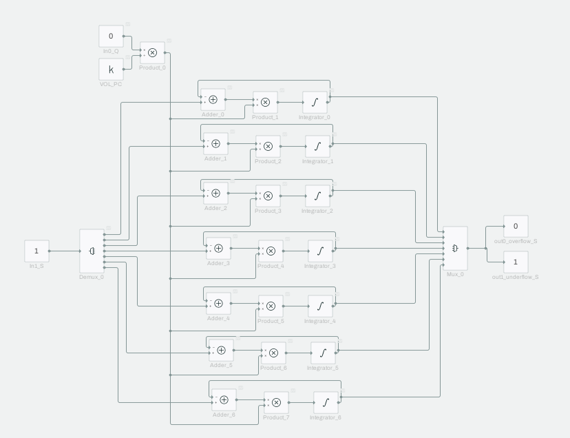 {width="5.0in" height="3.84375in"}
- Inside PC_X_Q submodel. The ODE is solved the same way as PC_S. However, the outputs are dependent on the PC removal efficiency to determine ratio of particulate concentration for overflow and underflow. Python script block is added to do this calculation.
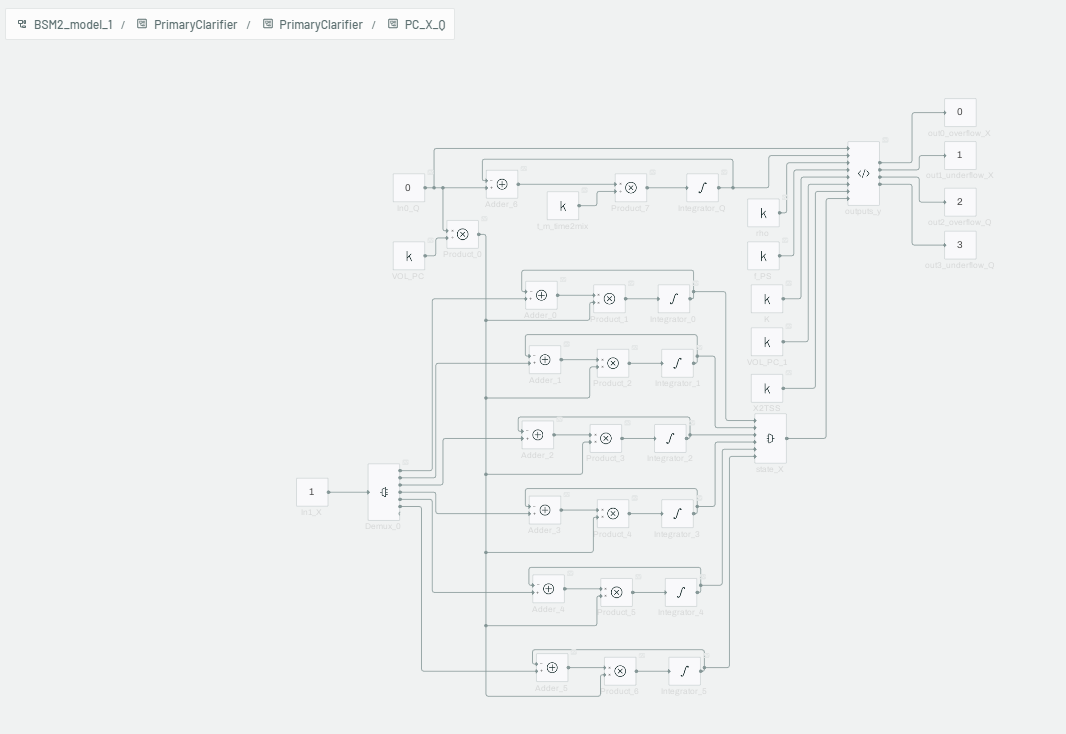 {width="5.0in" height="3.4479166666666665in"}
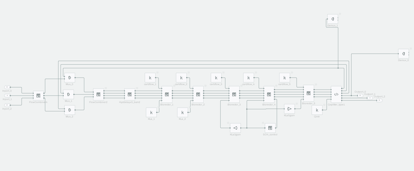
Activated Sludge
Qintr -- flow internally recycled
Combine flow block:
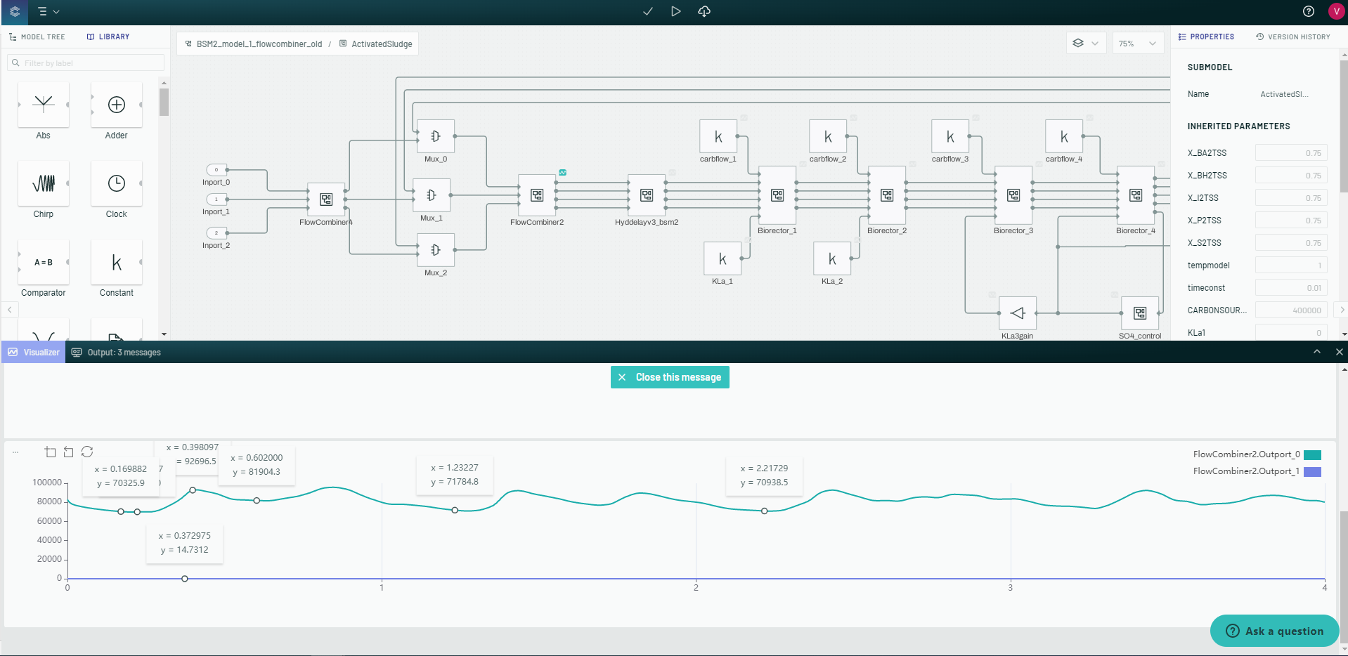
The flow coming out from combine flow block around 70,000 to 100,000. These values are lesser than ASinput from matlab the lowest value is 88,186.41.
 {width="6.5in" height="3.165277777777778in"}
Hyd_delay block:
Initial condition (XINITDELAY)
- Default value (unit: g/day)
 {width="5.0in" height="0.3229166666666667in"}
Same principle as hyd_delay applied for primary clarifier
Carboncombiner_bsm2:
- Combine carbon source flow with influent flow
Initial Conditions:
- No initial condition
Parameters:
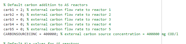
- CARBONSOURCECONC = 400,000 mg COD/l (gCOD/m\^3)
For state-space system:
U= input; X = state variable; y = output
Input:
- Input for carbon source (store as carbon1in/carb1, carbon2in/carb2, carbon3in/carb3, carbon4in/carb4, or carbon5in/carb5 for bioreactor 1 to 5)
 {width="1.5416666666666667in"
height="0.9479166666666666in"}
{width="1.5416666666666667in"
height="0.9479166666666666in"}
 {width="6.5in" height="1.5472222222222223in"}
Input for soluble block (u) = Si, Ss, So, Sno, Snh, Snd, Salk; Q
Input for particulate block (u) = Xi, Xs, Xbh, Xba, Xp, Xnd, TSS; Q
Input for flow and temperature (u) = Q and Temperature
ODE:
- No ODE
Output:
Soluble:
y(All except SS) =( u*u(Q))/(carbon flow + u(Q))
y(SS) = (u(SS)*u(Q) + carbonsourceconcentration*carbonflow)/(carbon flow + flow_rate(Q))
Particulate:
- y =u*u(Q)/(carbon flow + u(Q))
Flow:
- y(Q) = carbon flow + u(Q)
Temp:
- y(temp) = u(temp)
Bioreactor 1 (asm1_bsm2):
Parameters:
- XINIT1
 {width="6.5in" height="0.4409722222222222in"}
- PAR1
 {width="6.5in" height="0.3in"}
VOL1 = 1500 m\^3
SOSAT1 = 8 # Oxygen saturation concentration at 15 degC, based on BSM1
TEMPMODEL = 1 # type of temperature model
ACTIVATE = 0 # is used when added extract variables (the last five variables)
For state-space system:
U= input; X = state variable; y = output
Input:
Input for soluble block (u) = Si, Ss, So, Sno, Snh, Snd, Salk; Q
Input for particulate block (u) = Xi, Xs, Xbh, Xba, Xp, Xnd, TSS; Q
Input for flow and temperature (u) = Q and Temperature
KLa
{width="3.0729166666666665in" height="1.21875in"}
ODE:
Parameters:
- PAR1
{width="6.542179571303587in"
height="0.36800087489063865in"}
VOL = VOL1
SO_sat = SOSAT
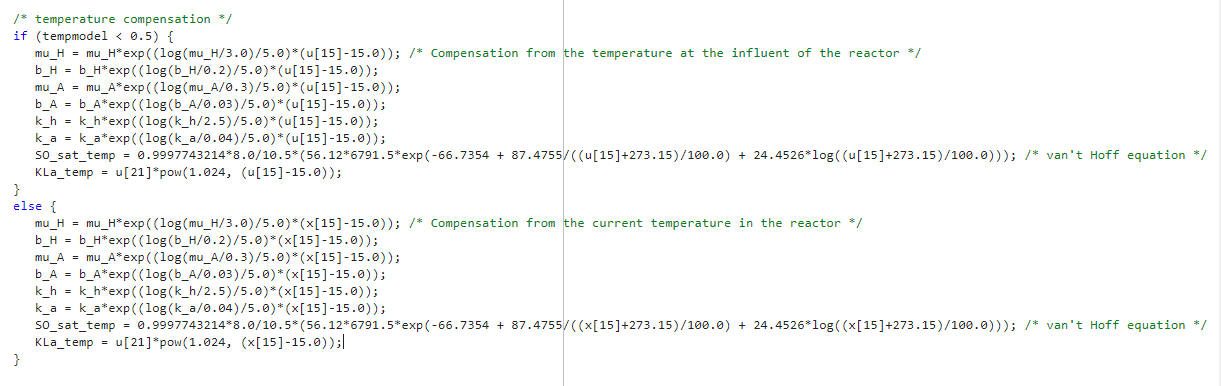 {width="6.5in" height="2.0548611111111112in"}
u[21] = Input_KLa
u[15] =Input_temperature
x[15] = state_temperature
reac1=0
For temperature: dx = (1.0/vol)*(u[Q]*(u[temperature]-x[temperature]))
For flow: dx =0
for soluble block and Particulate block (except TSS): Create tempX state:
All (except SO): dx = (1/vol)*(u[Q]*(u-x))
SO:
if u[21] \< 0 then x[SO] = abs(u[21]) (dx=0)
else: dx = 1/vol *(u[Q]*(u-x))
if x \< 0.00 => tempX = 0 else tempX = x
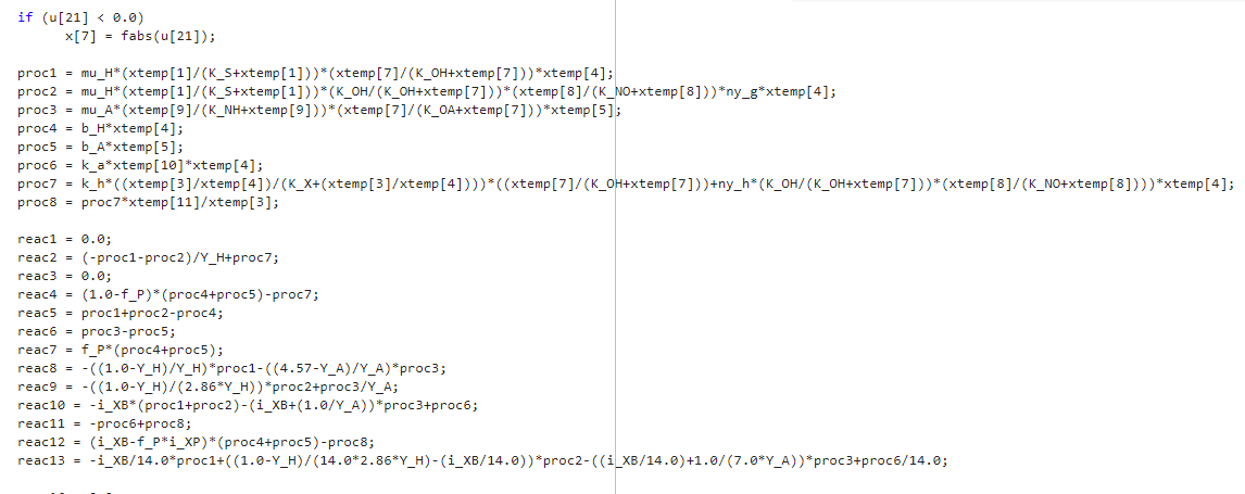
Use the tempX to find the parameter:
Input for soluble block (u) = Si(0), Ss(1), So(2), Sno(3), Snh(4), Snd(5), Salk(6); Q
Input for particulate block (u) = Xi (0), Xs(1), Xbh(2), Xba(3), Xp(4), Xnd(5), TSS(6); Q
 {width="6.5in" height="2.5805555555555557in"}
- Once you find the react 1 find the new x state:
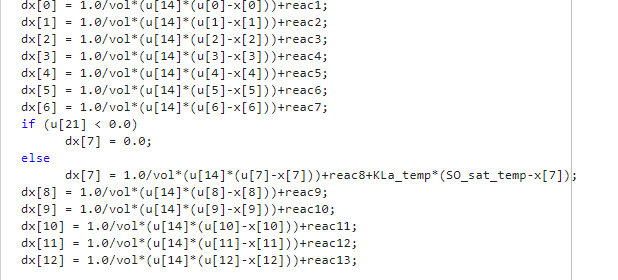 {width="6.4375in" height="2.9166666666666665in"}
for TSS:
- TSS: dx = 0
Output:
For Soluble:
- All (except SO): y(i) = x(i)
For Particulate:
For all (except TSS): y(i) = x(i)
TSS: y(TSS) = X_I2TSS*x(XI) + X_S2TSS*x(XS) + X_BH2TSS*x(XBH)+X_BA2TSS*x(XBA)+X_P2TSS*x(XP)
Flow: y(Q) = u(Q)
Temperature( Tempmodel=1): y(temp) = x(temp)
Bioreactor 2 (asm1_bsm2):
Parameters:
- XINIT2
 {width="6.28125in"
height="0.4580074365704287in"}
{width="6.28125in"
height="0.4580074365704287in"}
- PAR2
{width="6.5in" height="0.36564195100612423in"}
VOL2 = 1500 m\^3
SOSAT2 = 8
TEMPMODEL = 1
ACTIVATE=0
Bioreactor 3 (asm1_bsm2):
Parameters:
- XINIT3
 {width="6.5in" height="0.43194444444444446in"}
- PAR3
{width="6.5in" height="0.36564195100612423in"}
VOL3 = 3000 m\^3
SOSAT3 = 8
TEMPMODEL = 1
ACTIVATE=0
Bioreactor 4 (asm1_bsm2):
Parameters:
- XINIT4
 {width="6.5in" height="0.4270833333333333in"}
- PAR4
{width="6.5in" height="0.36564195100612423in"}
VOL4 = 3000 m\^3
SOSAT4 = 8
TEMPMODEL = 1
ACTIVATE=0
Bioreactor 5 (asm1_bsm2):
Parameters:
- XINIT5
 {width="6.5in" height="0.48333333333333334in"}
- PAR5
{width="6.5in" height="0.36564195100612423in"}
VOL5 = 3000 m\^3
SOSAT5 = 8
TEMPMODEL = 1
ACTIVATE=0
SO4_control:
Inputs:
SO (concentration of dissolved oxygen (g/m\^3))
SO from bioreactor 4 (ideal sensor without noise)
SO4 ref -- 2 g(-COD)/m\^3
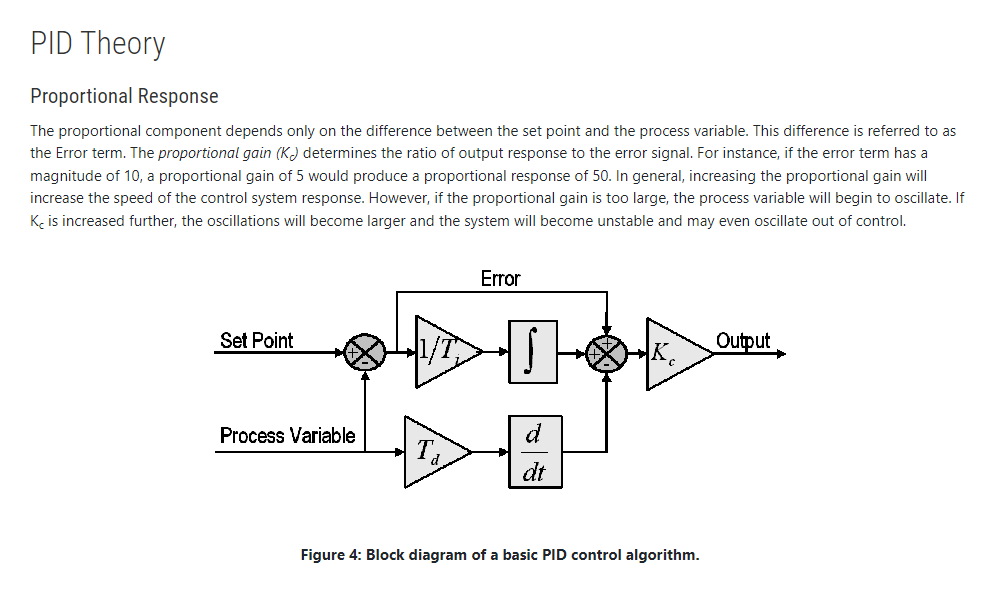
The primary control objective for the default strategies is to maintain the dissolved oxygen concentration in the fifth compartment at a predetermined set point value (2 g (-COD).m-3)
https://www.ni.com/en-ca/innovations/white-papers/06/pid-theory-explained.html: explain PID
 {width="6.5in" height="3.8625in"}
 {width="5.769250874890639in"
height="2.880497594050744in"}
{width="5.769250874890639in"
height="2.880497594050744in"}
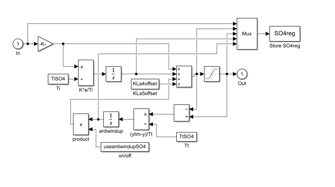
Figure 5. Matlab S04 control
PID part:
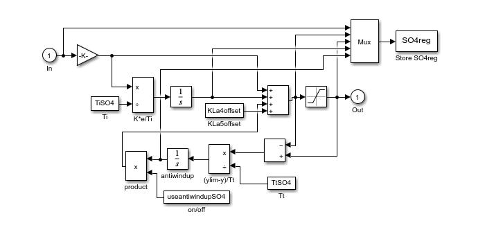
- Difference between set point (SO4_ref) and process variable (SO from biorector4) = in
<!-- -->
Proportional gain (Kp):
- K-gain = KSO4 = Kp=25
Integration gain (Ki):
K/TiSO4
TiSO4 = 0.002
Ki = 25/0.002 = 12500
Integrator block:
- Initial condition = SO4intstate = 0
Antiwindup part:
Tt = TtSO4 = 0.001
(ylim-y)/Tt = output of saturation block/Tt
Integration block:
Input: output of derivative gain
Initial condition = SO4awstate = 0
KLa4offset = 120
Saturation:
Upper limit = KLa4_max = 360
Lower Limit = 0
Integer rounding mode: floor
Product block to decide to use antiwindup part (set a variable to 1 if use, 0 if not)
{width="2.59375in" height="3.6041666666666665in"}
Settler
 {width="4.010503062117236in"
height="2.6985433070866143in"}
{width="4.010503062117236in"
height="2.6985433070866143in"}
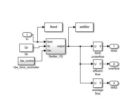
Figure 6. Settler block in Matlab
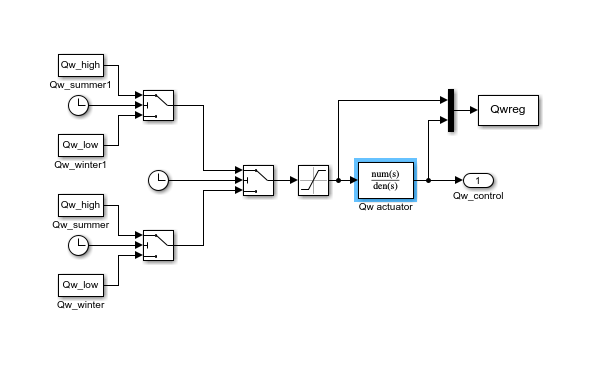
Qw_control block:
 {width="6.5in" height="1.9291666666666667in"}
 {width="5.388888888888889in"
height="2.8055555555555554in"}
{width="5.388888888888889in"
height="2.8055555555555554in"}
 {width="2.3958333333333335in"
height="1.0208333333333333in"}
{width="2.3958333333333335in"
height="1.0208333333333333in"}
Switch block 1 (Qw_summer1 and Qw_winter1):
- Clock is greater than or equal to 545.99999
Switch block 2(Qw_summer and Qw_winter):
- Clock is greater than or equal to 181.9999
Switch block 3(in the middle):
- Clock is greater than or equal to 363.99999
Saturation block:
Upper limit = Qw_max
Lower limit = 0
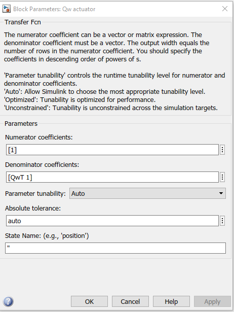
Qw actuator (Transfer Fcn block):
- QwT = 0.001
 {width="2.6822856517935256in"
height="3.570576334208224in"}
{width="2.6822856517935256in"
height="3.570576334208224in"}
Settler_1D
 {width="6.5in" height="2.3541666666666665in"}
Input:
Input for flow and temperature (u) = Q and Temperature
Input for soluble block (u) = Si, Ss, So, Sno, Snh, Snd, Salk
Input for particulate block (u) = Xi, Xs, Xbh, Xba, Xp, Xnd, TSS
Qr = 20648 m\^3/d (external recycle flow)
Qw_time_controller
 {width="6.201960848643919in"
height="0.25196522309711283in"}
{width="6.201960848643919in"
height="0.25196522309711283in"}
Figure 7. The order of input from Matlab
Parameters:
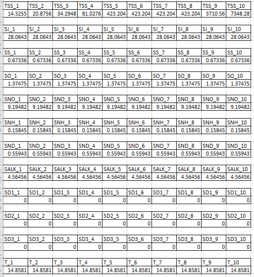
SETTLERINIT
From layer 1 to 10:
TSS: index[0,9]
Si: index[10,19]
Ss: index[20,29]
So: index[30,39]
Sno: index[40,49]
Snh: index[50,59]
Snd: index[60,69]
Salk: index[70,79]
3 Dummy variables: index [80,109]
Temperature: index[110,119]
 {width="5.447916666666667in"
height="5.9375in"}
{width="5.447916666666667in"
height="5.9375in"}
SETTLERPAR
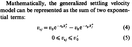
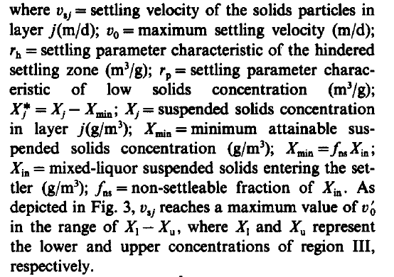
SETTLER is based on Takacs et al (1991) paper on a dynamic model of the clarification-thickening process
v0_max v0 r_h r_p f_ns Xt sb_limit
250 474 0.000576 0.00286 0.00228 3000 3000
v0 = maximum theoretical settling velocity (m/d)
v0_max = maximum practical settling velocity (m/d)
r_h = settling parameter associated with the hindered settling component of settling velocity equation (m\^3/g)
r_p = settling parameter associated with the low concentration and slowly settling component of the suspension (m\^3/g)
f_ns = non-settleable fraction of the influent suspended solids
Xt = threshold suspended solids concentration (g/m\^3)
Sb_limit =
Note: the settling velocity of solids particles in each layer has to be in between 0 and v0_max.
 {width="5.822916666666667in" height="1.40625in"}
 {width="4.225978783902012in"
height="1.5184601924759404in"}
{width="4.225978783902012in"
height="1.5184601924759404in"}
 {width="3.9631189851268593in"
height="2.7899212598425196in"}
{width="3.9631189851268593in"
height="2.7899212598425196in"}
DIM (dimension)
area = 1500 m\^2
height = 4 m
LAYER:
feedlayer = 5
nooflayer (number of layer) =10
MODELTYPE,
- Modeltype=0
 {width="6.5in"
height="0.7715277777777778in"}
{width="6.5in"
height="0.7715277777777778in"}
TEMPMODEL =1
ACTIVATE=0 (no dummy variable)
For state-space system:
Input (u) = 16 inputs + Qr and Qw (we do not have dummy variables)
State (x) =
Output(y) = 16 outputs for RAS (underflow, Q=Qr), 16 outputs for overflow (effluent flow, Q=Q_e), 16 outputs for WAS(wastage flow, Q=Q_w)
Calculated parameter:
Volume = area*height
eps =0.01
v_in (inflow velocity) = u[Q]/area
Q_f = u[Q]
Q_u = u[Qr]+u[Qw]
Q_e = u[Q] -- Q_u
v_up (upward flow velocity) = Q_e/area
v_dn (downward flow velocity) = Q_u/area
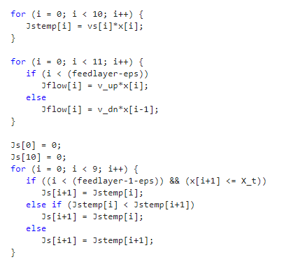
Calculate settling velocity for each layer (vs[i]):
For 10 layer
u[13] = u[TSS]
x[i] = suspended solid concentration in layer i (g/m\^3)
v0 = maximum theoretical settling velocity (m/d)
v0_max = maximum practical settling velocity (m/d)
the settling velocity of solids particles in each layer has to be in between 0 and v0_max.
 {width="3.9638845144356956in"
height="0.9891797900262467in"}
{width="3.9638845144356956in"
height="0.9891797900262467in"}
ODE:
- for 0 \<= i \< 10
 {width="4.947916666666667in"
height="1.6354166666666667in"}
{width="4.947916666666667in"
height="1.6354166666666667in"}
 {width="4.229166666666667in" height="4.0in"}
Output:
RAS
Soluble block (concentration from the bottom layer (10^th^))
Si = x[19]
Ss = x[29]
So = x[39] Use oxygen in return sludge flow
Sno = x[49]
Snh = x[59]
Snd =x[69]
Salk = x[79]
Particulate block:
All except TSS: y = u*gamma
TSS: y = x[9]?
Flow = Qr
Temp = x[119]? (tempmodel=1)
Overflow
Soluble block (concentration from top layer)
Si = x[10]
Ss = x[20]
So = x[30] Use oxygen in effluent flow
Sno =x[40]
Snh = x[50]
Snd = x[60]
Salk = x[70]
Particulate block:
Except TSS: y=u*gamma_eff
TSS = x[0]?
Flow = Q_e = u[Q] -- u[Qr] -- u[Qw]
Temp = x[110]?
Waste
Soluble block:
Si = x[19]
Ss = x[29]
So = x[39] Use oxygen in return sludge flow
Sno = x[49]
Snh = x[59]
Snd =x[69]
Salk = x[79]
Particulate block:
All except TSS: y = u*gamma
TSS: y = x[9]
Flow = Q_w=u[Qw]
Temp = x[119]? (tempmodel=1)
Internal TSS states
 {width="2.5729166666666665in"
height="3.28125in"}
{width="2.5729166666666665in"
height="3.28125in"}
Problem with Algebraic Loop
The algebraic loop is fixed using hyddelay block from matlab.
Output without delay block:
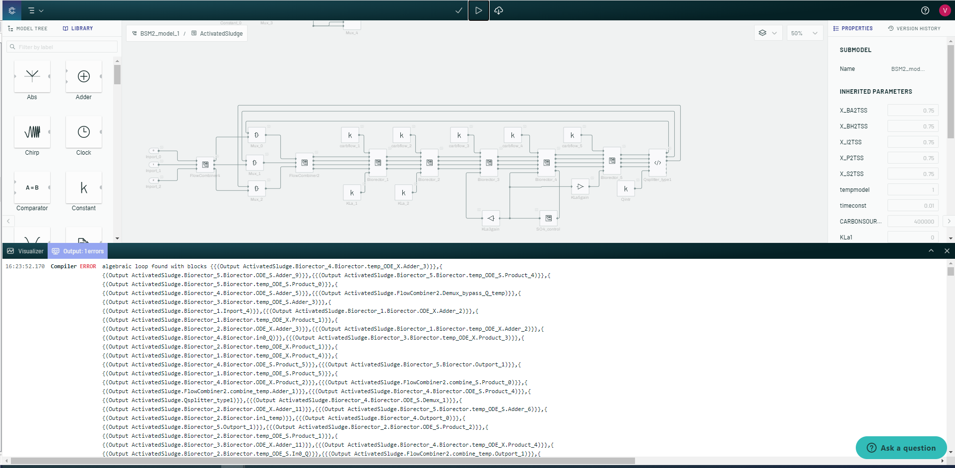 {width="6.5in"
height="3.1875in"}
{width="6.5in"
height="3.1875in"}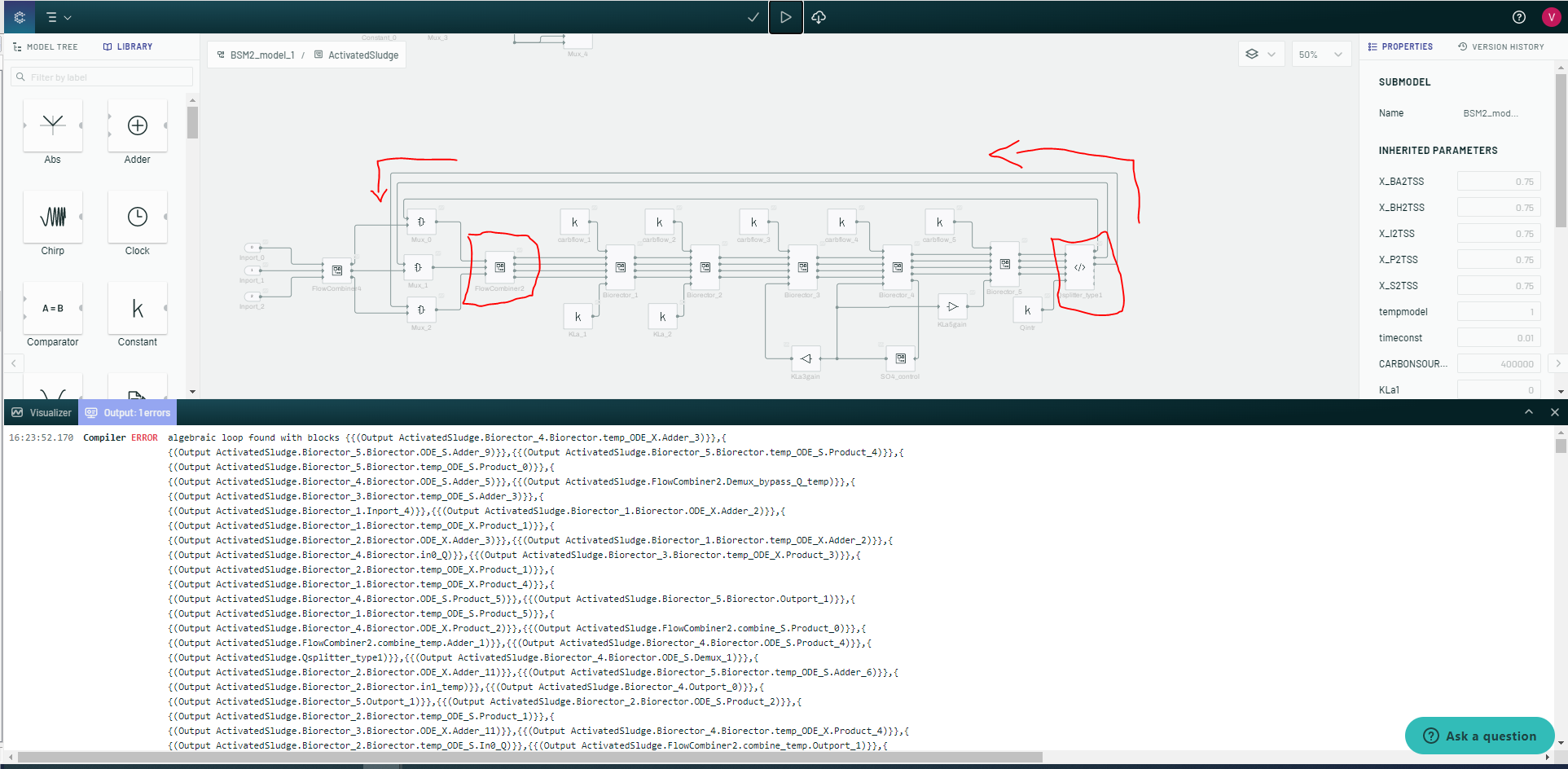 {width="6.495833333333334in"
height="3.1840277777777777in"}
{width="6.495833333333334in"
height="3.1840277777777777in"}
 {width="3.96875in" height="4.885416666666667in"}
 {width="6.5in" height="3.1805555555555554in"}
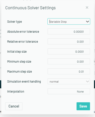
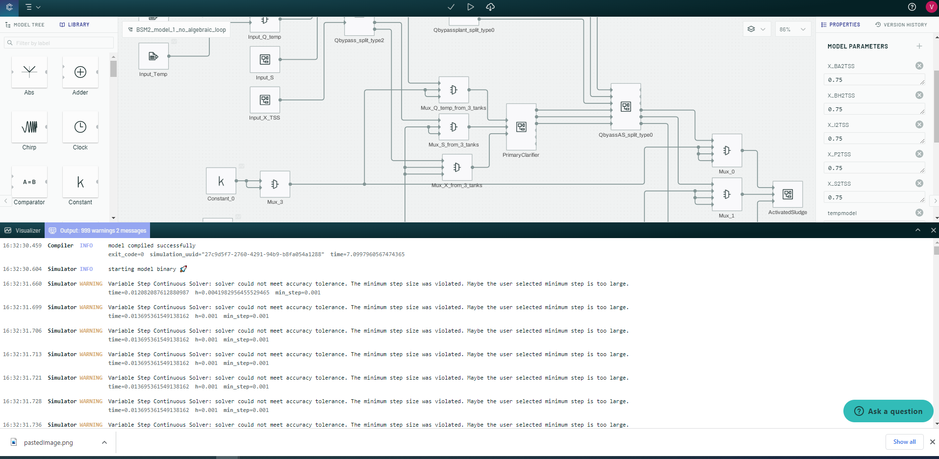
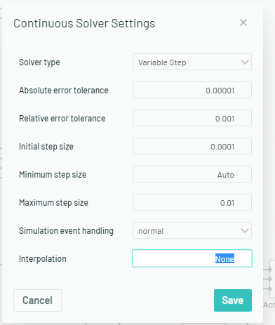
Change minimum step size from 0.001 to auto -> it works
Output using array of zero as a place holders instead of feeding the flow from Q split to the flow combiner block (interpolation = None)
 {width="2.5851192038495188in"
height="3.05334208223972in"}
{width="2.5851192038495188in"
height="3.05334208223972in"}
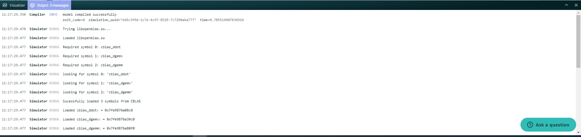
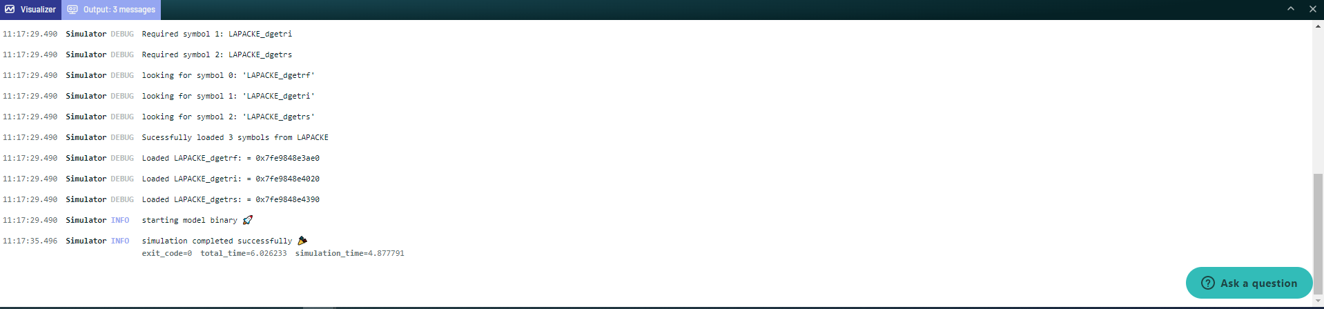
Output message:
 {width="6.5in" height="1.5402777777777779in"}
 {width="6.5in" height="1.5180555555555555in"}
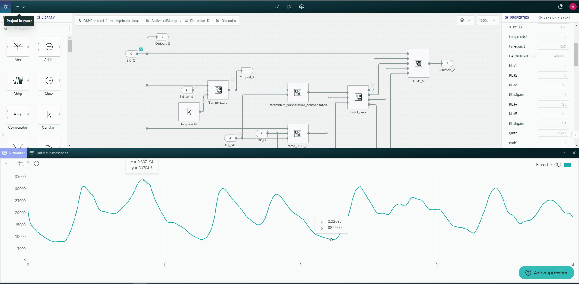
Flow from Bioreactor 5:
 {width="6.5in" height="3.1909722222222223in"}
TSS from Bioreactor 5:
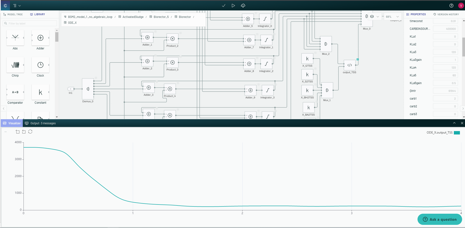 {width="6.5in" height="3.1875in"}
SO from Bioreactor 5:
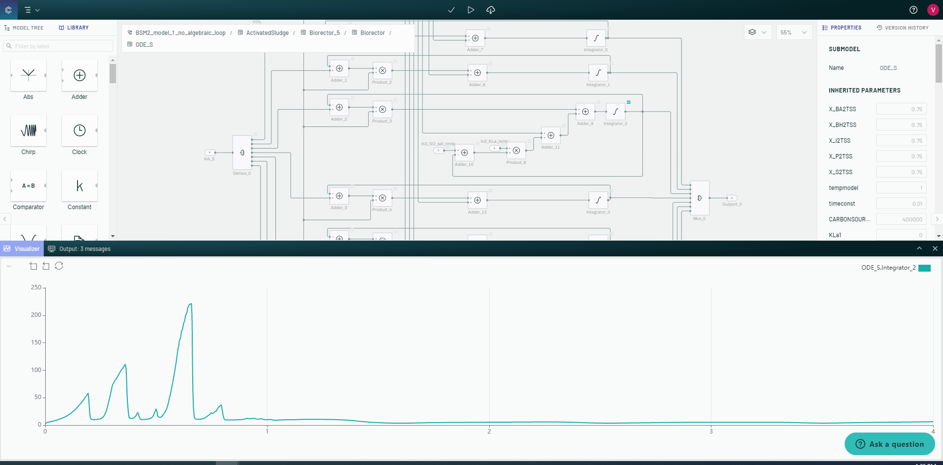 {width="6.5in" height="3.202777777777778in"}
Output using array of zero as a place holders instead of feeding the flow from Q split to the flow combiner block (interpolation = 0.002)
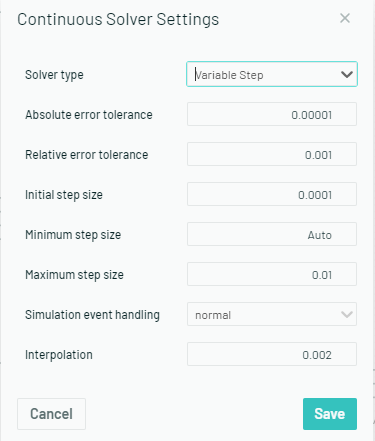 {width="3.90625in" height="4.59375in"}
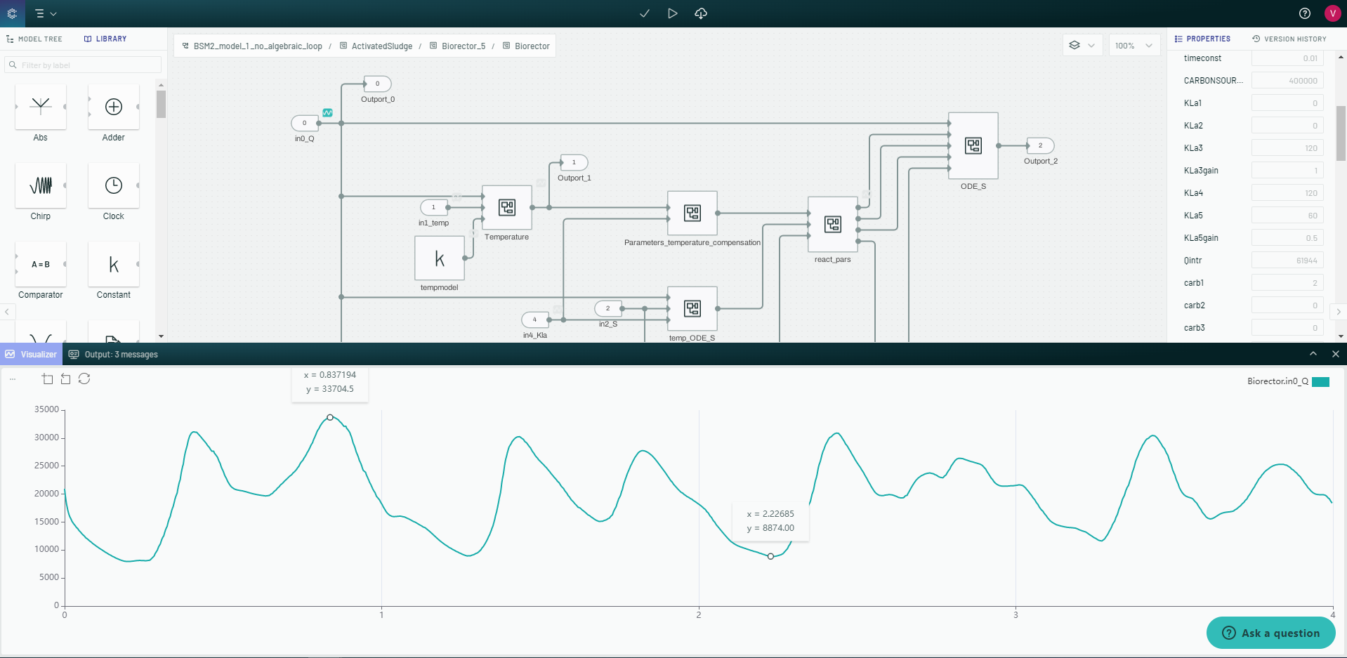 {width="6.5in" height="3.1756944444444444in"}
There is no difference in flow value when interpolation is set to None or 0.002
Controller:
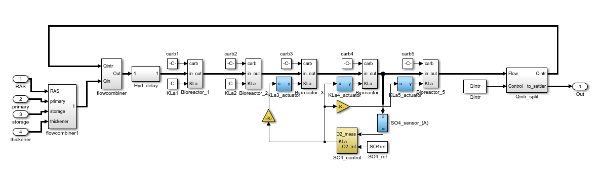
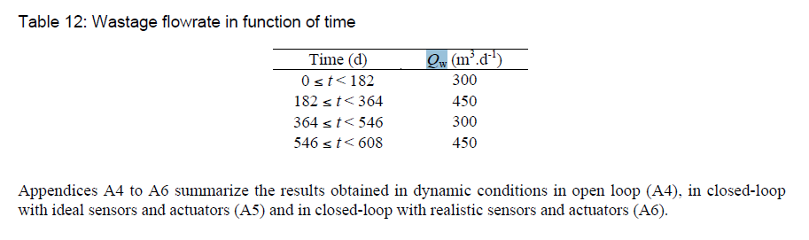
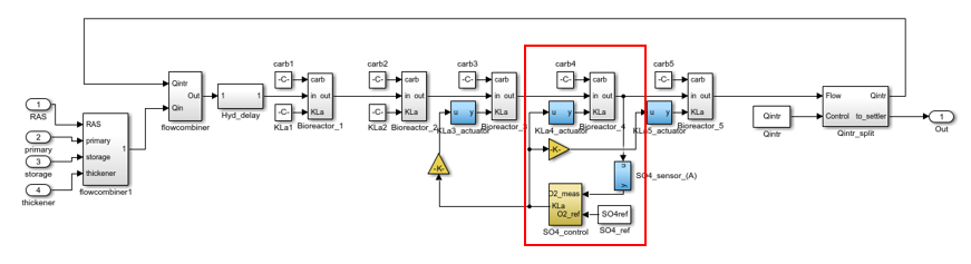
A default controller is proposed so the closed-loop simulation and the implementation of the evaluation criteria can be tested before the user implements his/her own control strategy. The primary control objective for the default strategies is to maintain the dissolved oxygen concentration in the fifth compartment at a predetermined set point value (2 g (-COD).m-3 is stored in the SO4ref variable) by manipulation of the oxygen transfer coefficient in the fourth reactor (shown in red box) in such a way that: KLa3 = KLa4; KLa5 = KLa4/2. Actuators models are used for the three oxygen transfer coefficients. The modeling principles of the sensors are given in Section 13 of this document. Furthermore, external carbon addition rate is 2.0 m3.d-1. Finally, two different wastage flow rates are imposed dependent on time of the year (Table 12), assuming day 0 is at the start of the 609 days period. For this reason a first-order filter (time constant = 0.0001 day) is added to simulate the response of the wastage pump.
Table 12: Wastage flowrate in function of time
 {width="2.5833333333333335in" height="1.25in"}
Appendices A4 to A6 summarize the results obtained in dynamic conditions in open loop (A4), in closed-loop with ideal sensors and actuators (A5) and in closed-loop with realistic sensors and actuators (A6).
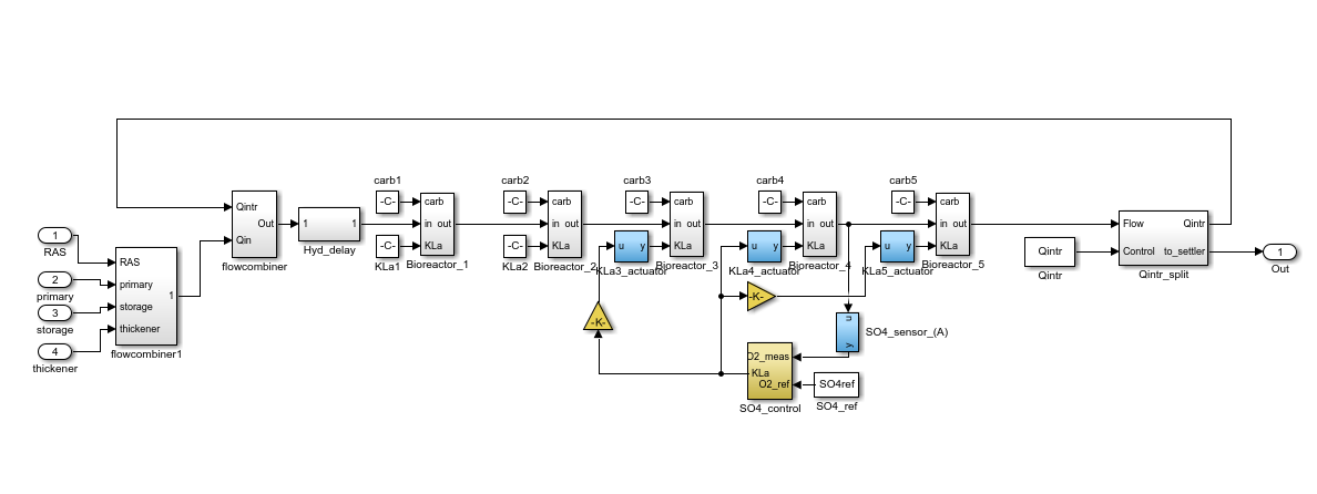 {width="6.5in" height="1.6348950131233595in"}
Figure 8.
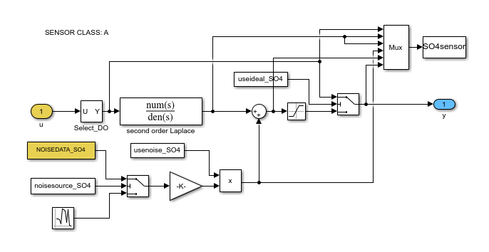 {width="6.5in" height="3.3541666666666665in"}
The original sensor signal u is transformed by a linear transfer function (block Transfer Fcn). This transfer function is used to implement the expected time response of the sensor. Real time behaviour of sensors is typically a combination of transport+delay time behaviour (or dead time) caused by sample transport and preparation and a first or higher order dynamics (time constants) caused by different reasons, e.g. a mixing tank.
To have a sensor model with the same response time, a series of equal first order delay transfer functions is assumed. The number of first order transfer functions in series (n) determines the ratio of delay time and response time (as defined in Figure 9). Table 16 shows the parameters for the response-time modelling (see specific sensor model) of the continuously operating sensors.
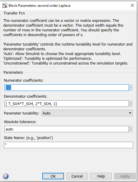
For the sensor class A a response time (tr) of 1 min and a system order of n = 2 is suggested. The assumed transfer function is:
 {width="6.5in" height="1.0666666666666667in"}
With =0.257 = tr /3.89, the ratio of the delay time to the rise time (Rtd/tr) is equal to 0.133. Thus the transfer
function is only a small fraction of the response time as typical for this sensor class.
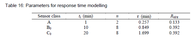 {width="6.5in" height="1.3958333333333333in"}
 {width="4.854166666666667in" height="6.40625in"}
 {width="6.5in" height="3.088888888888889in"}
Hi Brian, I have some questions on how I should build a controller in Collimator. So, the objective of the BSM2 model is to evaluate different control strategies, and one of the control strategies is to maintain the dissolved oxygen (DO) in the fifth reactor at 2g (-COD).m\^-3. They are doing that by manipulating the oxygen transfer coefficient (KLa4) in the fourth reactor in such a way that KLa3 = KLa4; KLa5 = KLa4/2. The figure below shows the layout of the model. The fourth reactor is enclosed in the red rectangle.
 {width="6.5in" height="1.76875in"}
In Matlab, they built a submodel to represent a sensor to measure the DO in the fourth reactor. The DO is transformed using a transfer function block. The transfer function block is used to implement the expected time response of the sensor.
For the DO sensor class A , a response time (tr) of 1 min and a system order of n = 2 is suggested. The assumed transfer function is:
{width="6.5in" height="1.0666666666666667in"}
{width="6.5in" height="3.3541666666666665in"}
DO controller is continuous PI type with anti-windup. The input of the DO controller is the difference between the measure DO from the sensor block and 2g (-COD).m\^-3 (the DO concentration set by the user)
{width="6.5in" height="3.088888888888889in"}
The first question is what approach I should do to get the transfer function for the sensor block, given that the sensor has a response time (tr) of 1 min and a system order of n =2. For your information, the sampling interval for each input from Data source is 15 minutes (0.0104 day).
The second question is what approach I should do to build the DO controller. Should I use the PID block?