BSM in MATLAB
A markdown file converted from Vannary's notes in
DOCXformat
Introduction
The benchmark is a simulation environment defining a plant layout, a simulation model, influent loads, test procedures and evaluation criteria. There are multiple vesion of BSM:
BSM1: combines nitrification with pregentrification, which is most commonly used for nitrogen removal. The control strategies are evaluated over periods of 14 days, with different weather conditions.
BSMLT: based on BSM1 but with a longer evaluation period (609 days)
BSM2: include BSM1 for the biological treatment of wastewater. The sludge treatment is taken into account.
Extension of BSM2
MATLAB files are available on request by contact Prof Ulf Jeppsson (ulf.jeppsson@iea.lth.se)
BSM2
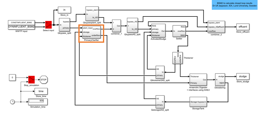 {width="6.5in" height="3.8881944444444443in"}
Note that for the BSM2 system there is rule saying that all influent flow above 60000 m\^3/d should be bypassed.
The plant is designed for an average influent dry-weather flow rate of 20,648.36 m3.d-1 and an average
biodegradable COD in the influent of 592.53 g.m-3. Its hydraulic retention time (based on average dry weather
flow rate and total tank volume -- i.e. primary clarifier (900 m3) + biological reactor (12,000 m3) + secondary
clarifier (6,000 m3) -- of 18,900 m3) is 22 hours.
Primary clarifier's volume ~ approximately 1000 m\^3
Flow = 100,000 m\^3/day
Time constant = 0.01 day
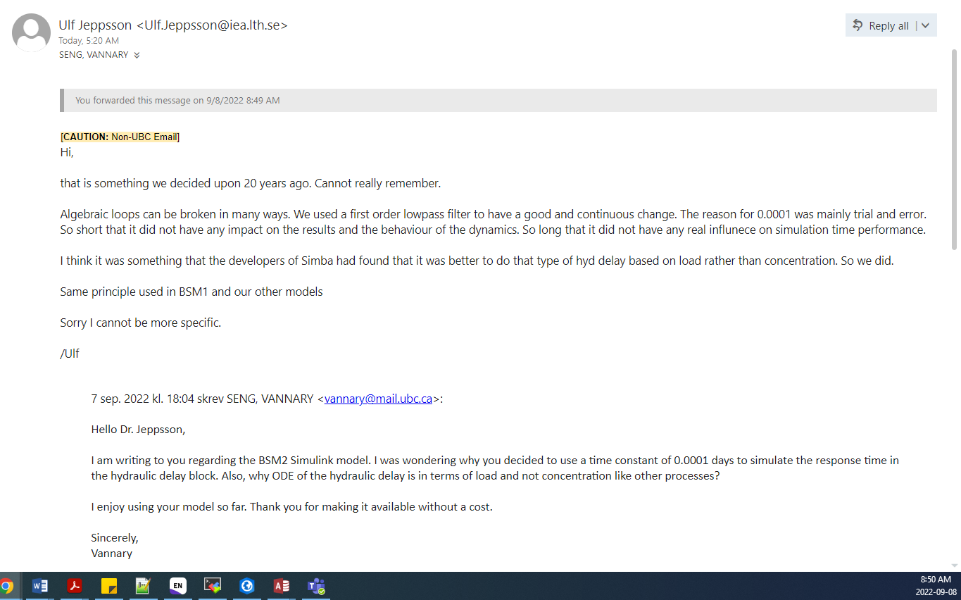
Matlab used 0.0001 day for time constant for hyddelay.
File Descriptions
Inside the BSM2_R2019b folder, there are three Simulink models:
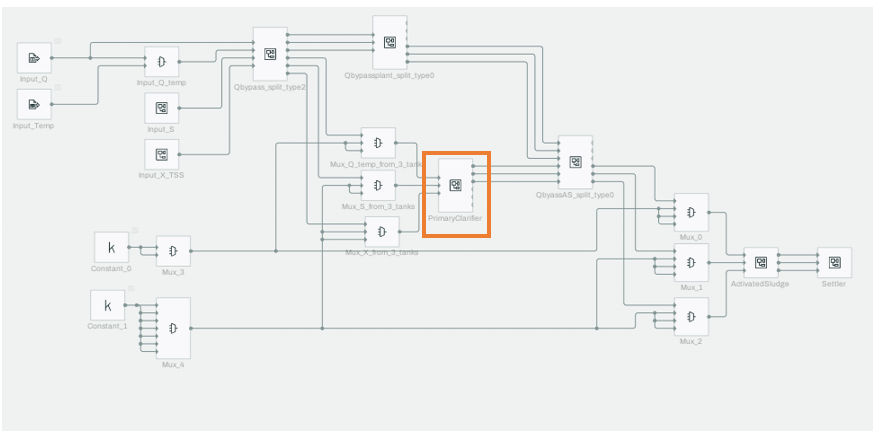 {width="3.881221566054243in"
height="4.188485345581802in"}
{width="3.881221566054243in"
height="4.188485345581802in"}
regent_bsm2.m and sensorinit_bsm2.m are only two files that you would need to modify when you add new sensors or new controllers. Parameter values for the controllers are defined in reginit_bsm2.m.
need to revise this
Data are stored in the following order in C file:
{width="6.5in" height="0.42916666666666664in"}
- The extra 5 indices are for five dummy variables.
Difference between BSM1 and BSM2
Volume of first and second bioreactors for BSM1: 1000 m\^3
Volume of first and second bioreactors for BSM2: 1500 m\^3
How to run the benchmark in MATLAB
Steps by Step
Command mexall_bsm2 (C-compiler)
Command bsm2_ss (simulate the plant without active control, in open loop using constant input data) to open Simulink window
Cd ./Influent_data/
Command create_noismatrix to create noise data for full 609 days of simulations
Command init_bsm2 to initiates all variables and parameters
In the Simulink simulation menu enter 200 or 500 days and select Run. Using constant influent data, open loop configuration, and solver ode15s to create steady state solution
Command stateset_bsm2 to store the steady state results that will be used to initialize all BSM2 models
Command load states_bsm2
Command bsm2_cl to open the Simulink window
In the Simulink simulation window, enter 609 for stop time for 609 days. Select Run. The system will be simulated 609 days forward in time using the dynamic influent data, the closed loop configuration including noise and non-ideal sensor models and solver ode45.
a. The steady state values obtained in this first simulation are subsequently used as initial values for simulations using the dynamic influent. From this starting point, BSM2 is simulated for 63 days (9 weeks, from t = 0 d to t = 63 d) with controls active to achieve a quasi or pseudo steady state based on the dynamic input data. This period is followed by 182 days of dynamic simulation (26 weeks, from t = 63 d to t = 245 d) in order to allow, for example, adaptive or model-based controllers enough time to adapt, estimate internal parameters or in some other way train the control algorithms. Finally, BSM2 is simulated for an additional 364 days (52 weeks, from t = 245 d to t = 609 d) and the output data generated during this last period (stored at 15-minute intervals) are used for plant performance evaluation.
16. Command save('name') to save the current workspace
Files to modify when running for different control strategies
Init_bsm2.m
asm1init_bsm2;

settler1dinit_bsm2;

hyddelayinit_bsm2;

primclarinit_bsm2;

thickenerinit_bsm2;

dewateringinit_bsm2;

storageinit_bsm2;

adm1init_bsm2; % also includes settings for AS/AD and AD/AS interfaces

reginit_bsm2;

load ./Influent_data/sensornoise_bsm2;

sensorinit_bsm2;

load ./Influent_data/constinfluent_bsm2;

load ./Influent_data/dyninfluent_bsm2;

\% General parameter for all subsystems

\% TEMPMODEL: 0 - influent wastewater temperature is just passed through
process reactors

\% 1 - mass balance for the wastewater temperature is used in

\% process reactors

\% Note: thickener and dewatering are ideal models, i.e. no impact since
T_out =

\% T_in, in flow splitters T_out = T_in and in flow combiners mass
balance based heat balance is always used.

TEMPMODEL = \[ 1 \];

\% to activate calculation of dummy states in settler, AS reactors and
storage tank set ACTIVATE = 1

ACTIVATE = \[ 0 \];
Reginit_bsm2.m
\%

\% Copyright: Ulf Jeppsson, IEA, Lund University, Lund, Sweden

\%

\% controll of bypassing options in BSM2

Qbypass = 60000; % type 2, everything above 60000 m3/d bypassed for
primary clarifier

Qbypasstype = 2;

Qbypassplant = 1; % type 0, all of this is also bypassed the AS system

Qbypassplanttype = 0;

QbypassAS = 0; % type 0, none of primary effluent bypassed for AS

QbypassAStype = 0;

Qthickener2AS = 0;% type 0, none of thickener effluent to AS, all to
primary

Qthickener2AStype = 0;

Qstorage2AS = 0; % type 0, non of storage tank effluent to AS, all to
primary

Qstorage2AStype = 0;

Qintrtype = 1; % type 1, specified flow internally recycled, default Qw
value in asm1init_bsm2.m

\% Default carbon addition to AS reactors

carb1 = 2; % external carbon flow rate to reactor 1

carb2 = 0; % external carbon flow rate to reactor 2

carb3 = 0; % external carbon flow rate to reactor 3

carb4 = 0; % external carbon flow rate to reactor 4

carb5 = 0; % external carbon flow rate to reactor 5

CARBONSOURCECONC = 400000; % external carbon source concentration =
400000 mg COD/l

\% Default KLa values for AS reactors

KLa1 = 0;

KLa2 = 0;

KLa3 = 120;

KLa4 = 120;

KLa5 = 60;

\% Default output pumping from storage tank

Qstorage = 0;

\% Default closed loop control of Qw

Qw_high = 450;

Qw_low = 300;

\% initiates parameters for all controllers in use

\% this file works together with sensorinit_bsm2.m

%continuous PI O2-controller

KSO4 = 25; %Amplification, 500 in BSM1 book

TiSO4 = 0.002; %I-part time constant (d = 2.88 min)), integral time
constant, 0.001 in BSM1 book

TtSO4 = 0.001; %Antiwindup time constant (d), tracking time constant,
0.0002 in BSM1 book

SO4intstate = 0; %initial value of I-part

SO4awstate = 0; %initial value of antiwindup I-part

SO4ref = 2; %setpoint for controller, mg (-COD)/l

KLa4offset = 120; %reasonable offset value for control around SO4ref

\% = controller output if the rest is turned off, (1/d)

useantiwindupSO4 = 1; %0=no antiwindup, 1=use antiwindup for oxygen
control

KLa3gain = 1.0; %gain for control signal to reactor 3

KLa5gain = 0.5; %gain for control signal to reactor 5

\% to be used for a Qintr controller of BSM1 type, should then be

\% sensorinit_bsm2 since it is an rudimentary \'actuator model\' similar
to QwT

%QintrT = T\*10;
Sensorinit_bsm2.m
\%

\% Copyright: Ulf Jeppsson, IEA, Lund University, Lund, Sweden

\%

\% initiates parameters for all sensors and actuators in use

\% this file works together with reginit.m

\% actuator limitations

\% aeration equipment capacity (also used by controller for anti-winup)

KLa1_max = 360; %maximum possible KLa value to reactor1

KLa2_max = 360; %maximum possible KLa value to reactor2

KLa3_max = 360; %maximum possible KLa value to reactor3

KLa4_max = 360; %maximum possible KLa value to reactor4

KLa5_max = 360; %maximum possible KLa value to reactor5

\% external carbon flow addition capacity (also used by controller for
anti-winup)

carb1_max = 5; %maximum possible external carbon flow rate to reactor1

carb2_max = 5; %maximum possible external carbon flow rate to reactor2

carb3_max = 5; %maximum possible external carbon flow rate to reactor3

carb4_max = 5; %maximum possible external carbon flow rate to reactor4

carb5_max = 5; %maximum possible external carbon flow rate to reactor5

\% pumping equipment capacity (also used by controllers for anti-windup)

Qintr_max = 5\*Qin0; %maximum pump capacity for Qintr (= 103240 m3/d)

Qw_max = 0.1\*Qin0; %maximum pump capacity for Qw (= 2064.8 m3/d)

Qr_max = 2\*Qin0; %maximum pump capacity for Qr (= 41296 m3/d)

Qstorage_max = 1500; %maximum pump capacity for Qstorage

QwT = T\*10; % time delay for artifiial Qw actuator (first-order filter)

\% actuator definitions BSM2 default strategy

\% KLa3 actuator, according to BSM definition, T90=4 min, n=2

T90_KLa3 = 4; %minutes

T_KLa3 = T90_KLa3/(24\*60)/3.89;

useideal_KLa3 = 0; %select ideal actuator or not (0=non-ideal, 1=ideal
(for testing)) for KLa3

\% KLa4 actuator, according to BSM definition, T90=4 min, n=2

T90_KLa4 = 4; %minutes

T_KLa4 = T90_KLa4/(24\*60)/3.89;

useideal_KLa4 = 0; %select ideal actuator or not (0=non-ideal, 1=ideal
(for testing)) for KLa4

\% KLa5 actuator, according to BSM definition, T90=4 min, n=2

T90_KLa5 = 4; %minutes

T_KLa5 = T90_KLa5/(24\*60)/3.89;

useideal_KLa5 = 0; %select ideal actuator or not (0=non-ideal, 1=ideal
(for testing)) for KLa5

%sensor definitions BSM2 deafult strategy, SO4 sensor

\% DO sensor, according to BSM definition (class A), T90=1 min, n=2

min_SO4 = 0; %lower measurement limit, mg/l

max_SO4 = 10; %upper measurement limit, mg/l

T90_SO4 = 1; %response time in minutes

T_SO4 = T90_SO4/(24\*60)/3.89;

std_SO4 = 0.025; %standard deviation of noise

NOISEDATA_SO4 = SENSORNOISEFULL(:, \[1 2\]); %define which column in
SENSORNOISE to use, column 1 = time

noiseseed_SO4 = 1; %noise seed for random generator (mean=0, std=1,
sample=1 per minute)

noisesource_SO4 = 0; %select noise source: 0=random generator,
1=predefined noisefile

usenoise_SO4 = 1; %select noise or not (0=no noise, 1=use noise) for DO
sensor

useideal_SO4 = 0; %select ideal sensor or not (0=non-ideal, 1=ideal (for
testing)) for DO sensor, overrides usenoise_SO5

\% SNO sensor, according to BSM1 definition (class B0), T90=10 min, n=8

\% min_SNO2 = 0; %lower measurement limit, 0 mg N/l

\% max_SNO2 = 20; %upper measurement limit, 20 mg N/l

\% T90_SNO2 = 10; %response time in minutes

\% T_SNO2 = T90_SNO2/(24\*60)/11.7724;

\% std_SNO2 = 0.025; %standard deviation of noise

\% NOISEDATA_SNO2 = SENSORNOISEFULL(:, \[1 3\]); %define which column in
SENSORNOISE to use, column 1 = time

\% noiseseed_SNO2 = 2; %noise seed for random generator (mean=0, std=1,
sample=1 per minute)

\% noisesource_SNO2 = 1; %select noise source: 0=random generator,
1=predefined noisefile

\% usenoise_SNO2 = 1; %select noise or not (0=no noise, 1=use noise) for
SNO sensor

\% useideal_SNO2 = 0; %select ideal sensor or not (0=non-ideal, 1=ideal
(for testing)) for SNO sensor, overrides usenoise_SNO2

\% for a KLa actuator use simulink model KLa_actuator, and change XXX in
file and simulink

\% T90_XXX = 4; %minutes

\% T_XXX = T90_XXX/(24\*60)/3.89;

\% useideal_XXX = 0; %select ideal actuator or not (0=non-ideal,
1=ideal)

\% for A class sensors use simulink model sensor A, and change XXX in
file and simulink

\% min_XXX = ?; %lower measurement limit

\% max_XXX = ?; %upper measurement limit

\% T90_XXX = 1; %respose time minutes

\% T_XXX = T90_XXX/(24\*60)/3.89;

\% std_XXX = 0.025; %standard deviation of noise

\% NOISEDATA_XXX = SENSORNOISEFULL(:, \[1 2\]); %define which column in
SENSORNOISE to use

\% noiseseed_XXX = 2; %noise seed for random generator (mean=0, std=1,
sample=1 per minute)

\% noisesource_XXX = 1; %select noise source: 0=random generator,
1=predefined noisefile

\% usenoise_XXX = 1; %select noise or not (0=no noise, 1=use noise) for
sensor

\% useideal_XXX = 0; %select ideal sensor or not (0=non-ideal, 1=ideal)
for sensor

\% for B0 class sensors use simulink model sensor B0, and change XXX in
file and simulink

\% min_XXX = ?; %lower measurement limit

\% max_XXX = ?; %upper measurement limit

\% T90_XXX = 10; %response time minutes

\% T_XXX = T90_XXX/(24\*60)/11.7724;

\% std_XXX = 0.025; %standard deviation of noise

\% NOISEDATA_XXX = SENSORNOISEFULL(:, \[1 3\]); %define which column in
SENSORNOISE to use

\% noiseseed_XXX = 2; %noise seed for random generator (mean=0, std=1,
sample=1 per minute)

\% noisesource_XXX = 1; %select noise source: 0=random generator,
1=predefined noisefile

\% usenoise_XXX = 1; %select noise or not (0=no noise, 1=use noise) for
sensor

\% useideal_XXX = 0; %select ideal sensor or not (0=non-ideal, 1=ideal)
for sensor

\% for C0 class sensors use simulink model sensor C0, and change XXX in
file and simulink

\% min_XXX = ?; %lower measurement limit

\% max_XXX = ?; %upper measurement limit

\% T90_XXX = 20; %response time minutes

\% T_XXX = T90_XXX/(24\*60)/11.7724;

\% std_XXX = 0.025; %standard deviation of noise

\% NOISEDATA_XXX = SENSORNOISEFULL(:, \[1 4\]); %define which column in
SENSORNOISE to use

\% noiseseed_XXX = 3; %noise seed for random generator (mean=0, std=1,
sample=1 per minute)

\% noisesource_XXX = 1; %select noise source: 0=random generator,
1=predefined noisefile

\% usenoise_XXX = 1; %select noise or not (0=no noise, 1=use noise) for
sensor

\% useideal_XXX = 0; %select ideal sensor or not (0=non-ideal, 1=ideal)
for sensor

\% for B1 class sensors use simulink model sensor B1, and change XXX in
file and simulink

\% min_XXX = ?; %lower measurement limit

\% max_XXX = ?; %upper measurement limit

\% T90_XXX = 10; %response time minutes

\% T_XXX = T90_XXX/(24\*60)/11.7724;

\% T0_XXX = 5/(24\*60); %sample time (minutes = 5)

\% std_XXX = 0.025; %standard deviation of noise

\% NOISEDATA_XXX = SENSORNOISEFULL(:, \[1 3\]); %define which column in
SENSORNOISE to use

\% noiseseed_XXX = 2; %noise seed for random generator (mean=0, std=1,
sample=1 per minute)

\% noisesource_XXX = 1; %select noise source: 0=random generator,
1=predefined noisefile

\% usenoise_XXX = 1; %select noise or not (0=no noise, 1=use noise) for
sensor

\% useideal_XXX = 0; %select ideal sensor or not (0=non-ideal, 1=ideal)
for sensor

\% for C1 class sensors use simulink model sensor C1, and change XXX in
file and simulink

\% min_XXX = ?; %lower measurement limit

\% max_XXX = ?; %upper measurement limit

\% T90_XXX = 20; %response time minutes

\% T_XXX = T90_XXX/(24\*60)/11.7724;

\% T0_XXX = 5/(24\*60); %sample time (minutes = 5)

\% std_XXX = 0.025; %standard deviation of noise

\% NOISEDATA_XXX = SENSORNOISEFULL(:, \[1 3\]); %define which column in
SENSORNOISE to use

\% noiseseed_XXX = 2; %noise seed for random generator (mean=0, std=1,
sample=1 per minute)

\% noisesource_XXX = 1; %select noise source: 0=random generator,
1=predefined noisefile

\% usenoise_XXX = 1; %select noise or not (0=no noise, 1=use noise) for
sensor

\% useideal_XXX = 0; %select ideal sensor or not (0=non-ideal, 1=ideal)
for sensor

\% for D class sensors use simulink model sensor D, and change XXX in
file and simulink

\% min_XXX = ?; %lower measurement limit

\% max_XXX = ?; %upper measurement limit

\% T0_XXX = 30/(24\*60); %sample time (minutes = 30)

\% std_XXX = 0.025; %standard deviation of noise

\% NOISEDATA_XXX = SENSORNOISEFULL(:, \[1 3\]); %define which column in
SENSORNOISE to use

\% noiseseed_XXX = 2; %noise seed for random generator (mean=0, std=1,
sample=1 per minute)

\% noisesource_XXX = 1; %select noise source: 0=random generator,
1=predefined noisefile

\% usenoise_XXX = 1; %select noise or not (0=no noise, 1=use noise) for
sensor

\% useideal_XXX = 0; %select ideal sensor or not (0=non-ideal, 1=ideal)
for

\% sensor
To-do list:
Train on
No knowledge of influent -> if you have missing feature can
How well our mode done with missing feature (missing one of the column) to predict the effluent
Can model accept Nan as input?
For example, if you are measuring the pump energy
Aretion plant unit instead of measuring oxygen unit as input.
Look it up if someone already done by using the dry model on again different dataset (rain and storm data)
Regret analysis- on dry model on rain and storm data vs rain model and storm model.
Climate change
Default setting
Parameter
TEMPMODEL = 1 Type of temperature mode (if = 1, T(out) is a first- order)
Qbypasstype = 2 Type of model to handle exceed flow
PAR_P: parameter for primary clarifier
PAR_P[0] = 0.65 Settler efficiency correction
PAR_P[1] = 0.85 Average CODpart/CODtot ratio
PAR_P[2] = 0.1250 N/A
PAR_P[3] = 0.007 Ratio of primary sludge flow rate to the influent flow
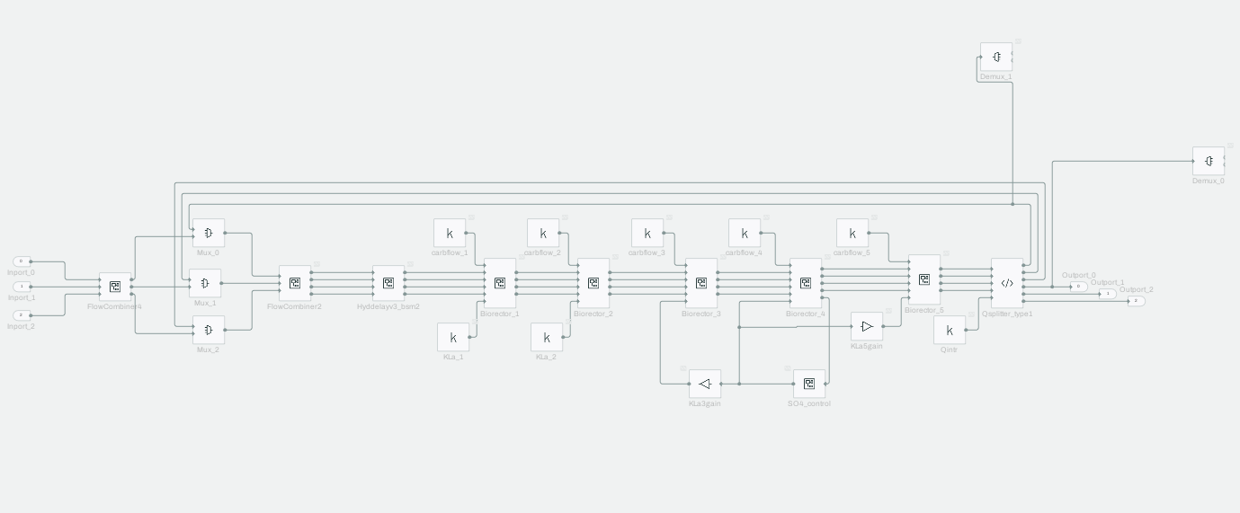 {width="6.5in" height="2.0861111111111112in"}
Email from Dr. Jeppsson regarding Hyddelay block
 {width="5.0in"
height="3.125in"}
{width="5.0in"
height="3.125in"}
Process flow diagram
After Having Steady state stored and commend mex all_bsm2 and have created noise data for 609 days.