GIS + Predictive model
Overview
This project, based in the District of North Vancouver, involves spatially mapping defect locations onto a GIS and developing predictive models to visually assess the probability of defects in sanitary pipes (or sewer mains) based on pipe characteristics.
This has 2 parts:
Defect Location Mapping to GIS: The first part involves mapping defect locations to a Geographic Information System (GIS). This step involves associating the geographical coordinates of defect locations in form of shape files with specific points or regions on QGIS.
Defect Likelihood Prediction Models: The second part focuses on creating predictive models based on different defect labels to estimate the probability of defects (binary outcome) occurring in a pipe. These models utilize pipe details as input and predict the likelihood of defects occurring within the pipe. In our case, we are using LightGBM to create prediction models. Predictions are made with the locations of the pipes expressed in rectangular as well as polar coordinates.
- The features that are primarily used for LightGBM training are:
'pipe_id', 'pipe_size', 'age', 'seg_material', 'pipe_shape', 'group_2' - The output feature is 1 unique value taken from
group_2. In the notebook, it isI.Note: group_2 is created based on
Codecolumn.
These notebooks are part of the gqc-utility-notebooks repo as cctvgis project and they are still in the dev branch.
LightGBM training overview
A binary model is trained for a selected defect label for predicting the existence of the selected defect.
- Model type: A binary classifier based on decision trees
- Input features:
pipe_size,age,seg_material(expanded through one-hot-encoding) - Unused input features: The code reveal that
pipe_shapehas been tested as an input feature. But not in the latest code. - Output data: Binary value for existence of a
selected defect label.- The notebook shared by Vannary has
Iforselected defect label. Iis acompressed-labelfor the defect label group: 'IS', 'IW', 'ID', 'IG'
- The notebook shared by Vannary has
Associated notebooks in gqc-utility-notebooks repo
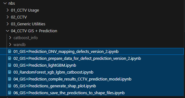
Currently there are 7 notebooks.
Dataflow diagram
Does not include all the notebooks yet. Data flow diagram link to all_notebooks(starting with notebook 1): https://general.gqc.com/people/Vishwanatha/CCTV/notebook_01
01_GIS+Prediction_DNV_mapping_defects_version_2.ipynb
This adds existing defects to a map and saves it as a shapefile using
geopandasCreates a
inspection_infoCSV with additional columns.
Here the material is being edited, as the material property coming from the shape files are wrong and updated with the property coming from metadata.
Condition data, headers, and list of videos are the following. Need to understand how these are created.
with working_directory(WORKING_DIR / CONDITION_DATA_DIR):
   cctv_header = pd.read_csv('CCTV_Headers.csv')
   cctv_detail = pd.read_csv('dnv_B_C_condition_data_with_remarks_col.csv')
   cctv_detail_full = pd.read_csv('CCTV_Details_sorted_by_jobnumber_distance_code_edit.csv')
   cctv_header_81 = pd.read_csv('combined_pipe_properties_84videos.csv')
   cctv_detail_81 = pd.read_csv('dnv_pacp_A_81_condition_data.csv')

with working_directory(WORKING_DIR / 'video_lists'):
   list_81_videos = pd.read_csv('DNV_PACP_81videos_edit.csv')
   list_videos = pd.read_csv('DNV_PACP_711_out_5238videos.csv')
Difference of columns between the input header file and the
Inspection info csv:

02_GIS+Prediction_prepare_data_for_defect_prediction_version_2.ipynb
03_GIS+Prediction_lightGBM.ipynb
This lightGBM notebook is replaced by the four notebooks described in the next section.
(NEW) Latest set of notebooks shared by Vannary
Content of the following 4 notebooks replace the step covered by
03_GIS+Prediction_lightGBM.ipynbabove. Some of the steps are only required as research and can be omitted in production. Check the next section on a proposed plan.
(RESEARCH)03_RandomForest_xgb_lgbm_catboost.ipynbThis tunes hyperparameters of four algorithms:
xgboost,lightGBM,catboost, andRFCand obtains the optimal model architecture.noteModel Architectures differ by:
- Algorithm:
xgboost,lightGBM,catboost,RFC - Sampling method: by
class weights,SMOTE/SMOTENC,RUS - Use internal categorization from model API:
Yes,No
- Algorithm:
(RESEARCH)04_GIS+Prediction_compile_results_CCTV_prediction_model.ipynbThis calculates the confusion matrix and the optimal threshold values.
(RESEARCH)05_GIS+Predictions_generate_shap_plot.ipynbVisualizes the result with
shapplots.06_GIS+Predictions_save_the_predictions_to_shape_files.ipynb
Trains a model, generates the predictions on test data, and writes the resultant predictions to shape files.
  input2{{"`BEST_MODEL_PARAMETER_DIR`
  (`pkl` files of models with optimal parameters)"}}

  input3{{"Shape files
  - Sanitary mainline
  - Sanitary history mainline
  Eg: mainline (CCTV/DNV/GIS/shapefiles/SanMain_shp/SanMain.shp)
      mainlinehist (CCTV/DNV/GIS/shapefiles/SanHistMain_shp/SanHistMain.shp)"}}

  model_file{{"(MODEL_DIR = WORKING_DIR / model_files/model_name.joblib)"}}

  output1{{"shape file WORKING_DIR / OUTPUT_SHAPE_FILE_DIR / SAVE_DIR / <shapefile_name>"}}

  subgraph 06_save_the_predictions.ipynb
     nb6_p1["Configure the model and train"]
     nb6_p2["Load Model and generate predictions on test data"]
     nb6_p3["Add pipe defect predictions to GIS"]

     nb6_p1 -.-> nb6_p2
     nb6_p2 -.-> nb6_p3
  end

  input1 --> nb6_p1
  input2 --> nb6_p1
  nb6_p1 --> model_file
  model_file --> nb6_p2
  input3 --> nb6_p3
  nb6_p3 --> output1
Latest .py file for notebook 7: /home/gqc/git/gqc/gqc-utility-notebooks/nbs_db/cctv_ml/07_cctv_nb.py
Latests .ipynb notebook for notebook 7: /home/gqc/git/gqc/gqc-utility-notebooks/nbs/04_cctv_ml/07_CCTV-defect-prediction-GIS.ipynb
Proposed production workflow
- Implement this proposal
This is the proposed workflow omitting
RESEARCHcomponents. As the steps are refined, the process can be streamlined for production.
More details on each notebook
mapping_defects_version_2.ipynb - Colab
Read shape files - Mainline and Manhole
Read condition data - Header and condition
cctv_header = pd.read_csv('CCTV_Headers.csv')
cctv_detail = pd.read_csv('dnv_B_C_condition_data_with_remarks_col.csv')
cctv_detail_full = pd.read_csv('CCTV_Details_sorted_by_jobnumber_distance_code_edit.csv')
cctv_header_81 = pd.read_csv('combined_pipe_properties_84videos.csv')
cctv_detail_81 = pd.read_csv('dnv_pacp_A_81_condition_data.csv')
Read video lists
list_81_videos = pd.read_csv('/content/drive/MyDrive/VS_Research/CCTV/DNV/Data/condition_data_csv/DNV_PACP_81videos_edit.csv')
list_videos = pd.read_csv('/content/drive/MyDrive/VS_Research/CCTV/DNV/Data/condition_data_csv/DNV_PACP_711_out_5238videos.csv')
PACP code groups to include and exclude were hardcoded as dictionaries.
Finding Upstream and downstream pipes
- for each pipe segment, get two end points and store in a list.
- for each pipe segment, get upstream and downstream invert.
- find the upstream and downstream pipe by matching end points or upstream with other pipe downstream invert values and vise versa. If upstream point or upstream invert value found no match, it is a upstream pipe. If downstream point or downstream invert value found no match, it is a downstream pipe.
- num_pipe_segments,upstream_pipe,downstream_pipe,Acronym,up_pipe_via_mh,down_pipe_via_mh are inserted and saved in Header condition data as v2.
Check for abnormal data in header_df by comparing with the data in newly added columns.
Map defects and save the filtered geoPandas dataframe as a shape file.
saved_directory = 'defect_location_version_2'
with working_directory('/content/drive/MyDrive/VS_Research/CCTV/DNV/GIS/shapefiles'):
if not os.path.exists(saved_directory):
   os.makedirs(saved_directory)

# defect_point_gdf_81.to_file(Path(saved_directory)/'DNV_81_pacp_code_points.shp')
Prepare_Data_For_Prediction_notebook - Colab
- Read Sanitary mainline and Sanitary history manline shape files (DNV).
- VS_Research/CCTV/DNV/GIS/shapefiles/SanMain_shp/SanMain.shp
- VS_Research/CCTV/DNV/GIS/shapefiles/SanHistMain_shp/SanHistMain.shp
- Read Data A
- PACP Defect codes shape file - VS_Research/CCTV/DNV/GIS/shapefiles/defect_location_version_2/DNV_81_pacp_defect_points.shp
- PACP All codes shape file - VS_Research/CCTV/DNV/GIS/shapefiles/defect_location_version_2/DNV_81_pacp_code_points.shp
- Header CSV file - VS_Research/CCTV/DNV/Data/feature_engineer_data/inspection_info_DNV_A_version_2.csv
- Rename material to the standard name in defect and all codes files. Then save the updated dataframes back as shape files.
- Read Data B
- PACP Defect codes shape file - VS_Research/CCTV/DNV/GIS/shapefiles/defect_location_version_2/DNV_B_C_pacp_wrc_defect_points.shp
- PACP All codes shape file - VS_Research/CCTV/DNV/GIS/shapefiles/defect_location_version_2/DNV_B_C_pacp_wrc_code_points.shp
- Header CSV file - VS_Research/CCTV/DNV/Data/feature_engineer_data/inspection_info_DNV_B_C_version_2.csv
- Detail CSV - VS_Research/CCTV/DNV/Data/feature_engineer_data/condition_data_DNV_B_C_version_2.csv
- Rename material to the standard name in defect and all codes files. Then save the updated dataframes back as shape files.
lightGBM - Colab
- Read the training CSV (CCTV/DNV/Data/feature_engineer_data/input_DNV_A_B_C.csv')
- One hot encoding the labels
- train and test along with different accuracy metric calculations
- Create a shape file with the predicted data
Next steps
- See if Deven has the notebooks in his local and figure out what is what.
- Only the first notebook was found in his laptop. That was also not run as seen from the cell outputs.
- Deven should have Q-GIS installed in his machine and we should be able to load the GIS output from the first notebook.
- Yes and working
- What features are used in the lightGBM?
Notebooks provided by Vannary
- Mapping defects
- For DNV : mapping_defects_version_2
- For others: METRO_mapping_defect_location_to_GIS.ipynb (This is found as an email attachment in Deven's inbox. Not tested)
- Prepare_Data_For_Prediction_notebook: Prepare_Data_For_Prediction_notebook_version_2
- lightGBM: lightGBM