Run Chama Notes

File Check

The current Generate Chama inputs from the SWMOPT2 is the same as generate Chama inputs from the gold standard of SWMOPT1. I compared the files to make sure that I was using the correct file, as the SWMOPT2 had not been running Generate Chama inputs.py I have set a testing called gold standard that in SWMOPT2. I will be running the python file generate_chama_inputs.py from this file as both this and the chama_opt.py file have config.json files that are needed to run the python files. I have only made the changes on my machine at the moment.

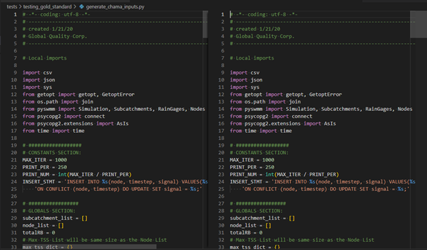
Figure 1: Verification of Chama Code

Generating the Signals File

Currently We are generating Chama inputs based on the rain gages. The rainfall timeseries are as follows:

• 0.1-in
• 0.23-in
• 2-yr
• 10-yr
• 100-yr

1st thing I am looking at is how the files change when we are using different amounts of rain.
Changing the rain gages does change the signal csv.

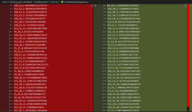
Figure 2: Signal Differences with rainfall changes

I have created the a folder for each of the generate Chama runs.
They contain the inp file and the output files from the Generate Chama Runs.

Figure 3: File folders for rainfall

I have also renamed the signal files so that I can easily run them. The next bullet list is the 1st timestamp of each of the signal files.
I have named them the same thing that the timeseries rain are named in the INP file. I am assuming the 2 year, 10 year and 100 year are named as such due to the high volume only happening every 2, 10 and 100 years.

• 0.1 in
  • J10,22,2.0910485232713576
  • J11,22,2.0828426270594953
• 0.23 in
  • J9,10,2.5694485655560255
  • J10,10,2.718904052756857
  • J11,10,2.736918435119016
  • J12,10,2.630697875234519
  • J14,10,2.5582804901947642
• 2 yr
  • J9,1,10.15511566547578
  • J10,1,10.384213086899816
  • J11,1,10.421506948668663
  • J12,1,10.28973202493085
  • J14,1,10.265701608700342
• 10 yr
  • J9,1,10.213059891584523
  • J10,1,10.530425444457743
  • J11,1,1.1592002279570526
  • J12,1,10.397314964788313
  • J14,1,10.360578164529125
• 100 yr
  • J9,1,10.321497008517735
  • J10,1,10.760783778588449
  • J11,1,1.4024443399073703
  • J12,1,10.597647652703323
  • J14,1,10.531721097464864

Just looking at the signal files I am seeing some things to note.

1. The signals are ordered by time they are added and not by node name. But once they are added into the time they are then ordered by node name.
2. Once a concentration has reached the node then we get concentration for that node at each timestamp.
   1. So it is detected fastest at the locations that show up first in the signals file?
   2. If so the fastest nodes are as follows:
      1. J10 and J11 show up in the 1st timestamp every time.
         1. For fast detection the J10 and J11 should be looked at.
         2. But J9, J12, and J14 are also good nodes if you have more sensors.
      2. The more rain I have the faster the contamination is measured.
   3. Although it seems like after a certain amount of rain the concentration in the rain gage even out there is not much difference between 2 years, 10 years, and 100 years.

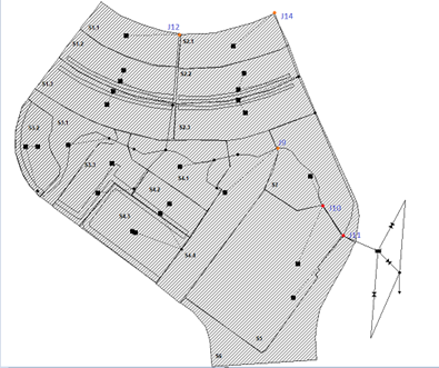
Figure 4: Nodes found in the 1st timesteps of the signals

Chama Outputs

Now I am going to start looking at the output of the Chama outputs. These were just showing up in the window before so I added some code that would allow them to be fed out into a CSV so I could get the data. Chama writes the data out in Panda’s data frames so it was a quick adding of a code line at each of the print statements to get the data in a CSV. Also, when a data frame is printed out the first few lines are printed then … and then the last few lines so not the best method of looking at the data to analyze. We were printing out 5 statements from chama_opt.py so we now have 5 files that I generate from this project.

1. detection_time_stats.csv
2. detection_times.csv
3. min_detection_time.csv
4. new_scenario.csv
5. scenario_time.csv

Detection Times

This data is generated by chama.impact.extract_detection_times(signals, sensors_dict) and it according to the documentation Chama Docs does the following:

1. Returns detection times from a signal and group of sensors.
2. The inputs are as follows:
   1. signal (pandas DataFrame) – Signal data from the simulation. The DataFrame can be in XYZ format (with columns named ‘X’,’Y’,’Z’,’T’) or Node format (with columns named ‘Node’,’T’) along with one column for each scenario (user defined names).
   2. sensors (dict) – A dictionary of sensors with key:value pairs containing {‘sensor name’: chama Sensor object}
   3. interp_method ('linear', 'nearest', or None) – Method used to interpolate the signal if needed. A value of ‘linear’ will use griddata to interpolate missing sample points. A value of ‘nearest’ will set the sample point to the nearest signal point within a minimum distance of min_distance. If there are no signal points within this distance then the signal will be set to zero at the sample point. Note that interpolation is not used when the signal is in Node format.
   4. min_distance (float) – The minimum distance when using the ‘nearest’ interp_method
3. This method returns det_times (pandas DataFrame) – DataFrame with columns ‘Scenario’, ‘Sensor’, and ‘Detection Times’.

The output of the detection times looks like:

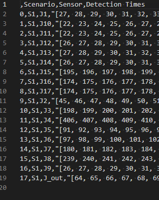
Figure 5: 0.1 inch start detection time

The start of the times seem to match up to what is in the signal file so Like the signal file the more rain added to a certain threshold the faster the detection will be. The larger the concentration the longer we have the contaminate detection for Most in this example still have contaminate at the end of the simulation but some do not. This means we would be able to model when the contaminate plume is out of the area and when it would be safe to use the water at some locations.

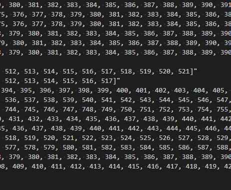
Figure 6: 0.1 inch end detection time

We could increase the simulation time to see how long it would take to get all of the contaminate out of the system. Something that was noticed was that while adding more water allowed for a faster detection it did not make the washout of the contaminate faster in fact for the 10 and 100 years simulation all the contaminate was still in the water at the end of the simulation.

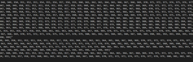
Figure 7: 100 years end detection time

This might be because we are using dirty rain as our contaminate process. This will be something to investigate when we start looking into how to model a contaminate. With dirty rain the more rain we have the faster the detection but also the longer we can detect the rain. A next step would be to review the how dirty rain works in SWMM as it has been a while since I have looked at it. I would like to check and see if it is a proportional contaminate to rain or if it is a set contaminate that is not dependent on how much rain we have. I suspect it is former.

Detection Time Stats

This data is generated by chama.impact.detection_time_stats(det_times) and it according to the documentation Chama Docs does the following:

1. Returns detection times statistics (min, mean, median, max, and count).
2. The inputs are detection_times (pandas DataFrame) – Detection times for each scenario-sensor pair. The DataFrame has columns ‘Scenario’, ‘Sensor’, and ‘Detection Times’, see detection_times.
3. The method returns det_t (pandas DataFrame) – DataFrame with columns ‘Scenario’, ‘Sensor’, ‘Min’, ‘Mean’, ‘Median’, ‘Max’, and ‘Count’.

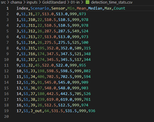
Figure 8: 0.1 inches detection statistics

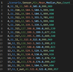
Figure 9: 0.23 inches detection statistics

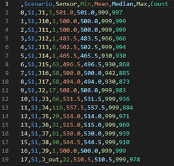
Figure 10: 2 years detection statistics

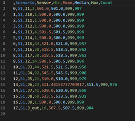
Figure 11: 10 years detection statistics

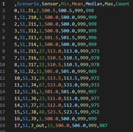
Figure 12: 100 years detection statistics

Minimum Detection Time

This data is generated by taking the minimum values from the detection time stats. Extract the minimum detection time from the from the Detection time stats.

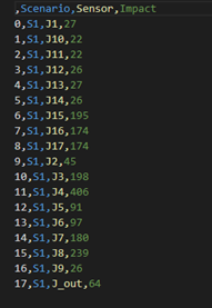
Figure 13: Minimum Detection Time

New Scenario and Scenario Time

This data is generated by scenario_time, new_scenario = chama.impact.detection_times_to_coverage(det_times, coverage_type=coverage_type, scenario=scenario)

1. Converts a detection times DataFrame to a coverage DataFrame. The returned coverage DataFrame can be used for input to a CoverageFormulation.
2. The inputs are as follows:
   1. detection_times (pandas DataFrame) – Detection times for each scenario-sensor pair. The DataFrame has columns ‘Scenario’, ‘Sensor’, and ‘Detection Times’, see detection_times.
   2. coverage_type ('scenario' or 'scenario-time') – Sets the coverage type: ‘scenario’ (the default value) builds lists of which scenarios are detected/covered by each sensor ignoring the time it was detected, ‘scenario-time’ treats every scenario-time pair as a new scenario and builds lists of which of these new scenarios are detected/covered by each sensor thereby calculating coverage over all scenarios and times.
   3. scenario (pandas DataFrame) – This is an optional argument which should be provided only if the coverage_type is ‘scenario-time’ and the user wants to propagate a scenario’s undetected impact and probability to the new ‘scenario-time’ scenarios. This DataFrame contains three columns, ‘Scenario` is the name of the scenarios, ‘Undetected Impact’ is the impact if the scenario goes undetected and ‘Probability’ is the probability or weighting of each scenario.
3. The values that are returned are
   1. coverage (pandas DataFrame) – DataFrame with columns ‘Sensor’ and ‘Coverage’ where the ‘Coverage’ column contains a list of the scenarios/entities detected by a sensor. Aka scenario time in our program.
   2. new_scenario (pandas DataFrame) – DataFrame returned if coverage_type is ‘scenario-time’ and a ‘scenario’ DataFrame was provided. The columns in this DataFrame match those in the provided ‘scenario’ DataFrame

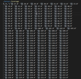
Figure 14: Scenario Time

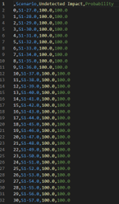
Figure 15: New Scenario

Conclusions on modifying the INP file

So far the changes made to chama have been through the INP file in order to change the amount of rain given in each simulation. This is something that needs to be taken into account and when constructing the testing and optimization. The testing and optimization will include multiple rain gages with differing amount of rain going to different locations. It may also be used to add in the contaminate into the simulation. We currently use 'dirty rain' to get the contaminate into the simulation. By have an contaminated rain gage and only assigning it to a specified area in the network we might be able to run a simulation similar to a dirty bomb. Sudhir and I will need to discuss this to flesh it out. This is not the only way we can modify a simulation in fact we have a config file what has several inputs that we can modify with chama_opt.py. This will be reviewed in the next section.

Next Steps for the INP file:

• talk to Sudhir about multiple rain gages in a simulation to simulate something happening only in 1 area of a network.
  • This may be a way to simulate things like a dirty bomb with rainfall if only one section of the network is getting a contaminate we can see how that effects the simulation.
• Review how 'dirty rain' works. I know that the contaminate is added to the rain. Is it a fixed amount of contaminate over a specified time regardless of rainfall volume or is the amount of rainfall directly proportional to the amount of rain. So more rain = more contaminate. This didn't matter when we had only one rain gage but it will if we do the multiple rain gages.
• Time both generate_chama_inputs.py and chama_opt.py so we can have a comparison for Banklick.
• Run Banklick at least 1 time so we know how long the runs are going to take.
• Look into other methods to introduce a contaminate into a network in SWMM simulation.
  • Buildup and washoff
  • Look into other ways

Json Config inputs

Figure 16: Inputs from the config.json file

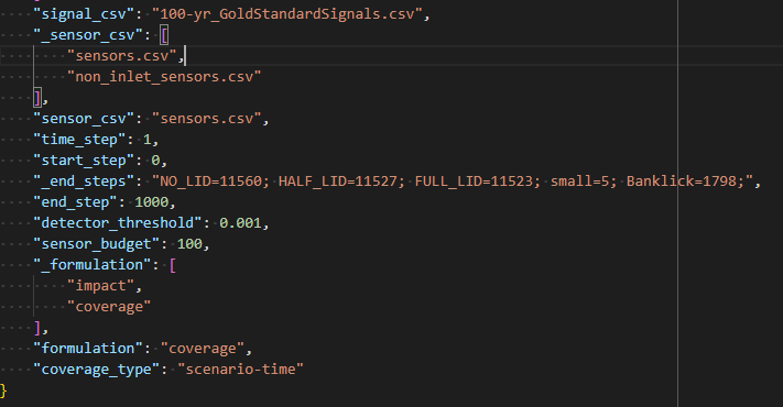
Beyond modifying the INP file there are also several modifcations we can make to a chama run by modifying the json config inputs. These changes will only require us to run chama_opt.py as well.

time_step

The length of the time step simulation currently set to 1. I need to verify what the time step actually stands for.

start_step

How far into the simulation should the optimization start. Currently set to zero or the start of the simulation.

end_step

How far into the simulation should the optimization end. Currently set to 1000. This is why all the results end either after there is no longer any contaminate detected or at step 999 since the timestep starts at 0.

_end_steps

I need to see if this is being used anywhere.

detector_threshold

How much contaminate is needed before it can be detected. Currently set to 0.001.

formulation

impact

According to Chama Read the Docs: The Impact formulation is used to determine optimal sensor placement and type that minimizes impact, where impact can be the sensor’s detection time or some other measure of damage

coverage

According to Chama Read the Docs: The Coverage formulation is used to place sensors that maximize the coverage of a set of entities, where an entity can be a scenario, scenario-time pair, or geographic location.

coverage_type

This is also part of the Impact assessment.

Impact assessment extracts the impact of a particular sensor detecting a particular scenario. Impact can be measured using a variety of metrics such as time to detection, population impacted, or volume of contaminant released before detection. Additionally, these impact metrics can be used to define when a sensor covers a particular scenario for use in coverage-based optimization formulations.

Scenario coverage

With scenario coverage, a scenario is the entity to be covered. A scenario is considered covered by a sensor if that sensor detects that scenario at any time.

Scenario-time coverage

With scenario-time coverage, the entities to be covered are all combinations of the scenarios and the detection times. This type of coverage gives more weight to sensors that detect scenarios for longer periods of time.